Turn Conditional Formatting On and Off (Show or Hide Conditional Formatting)
Simply put, there are two ways to turn Conditional formatting On and Off. The manual way will take you to the Home/Conditional Formatting/Manage Rules… window where you can delete the rules you want. But then there is an elegant way of doing this, that makes you look like an Excel Guru and that’s the one we will be learning here. We will achieve this with the use of Conditional Formatting. It’s funny and slightly “cannibalistic” since we will use Conditional Formatting to turn Conditional Formatting on and off, but it’s a very efficient and elegant way of doing this!
So here it is, the whole article will get you there in three stages. If you are already familiar with some just jump ahead to the part that interests you. The three parts will be:
-
Creating the Conditional Formatting rule, that we will turn on and off
-
Creating the rule with conditional Formatting that will enable us to turn the first rule on and off
-
Fixing all the settings in order for the toggling of Conditional Formatting to work.
Creating the original rule with conditional Formatting
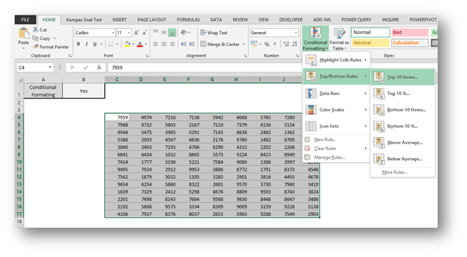
Here the original rule is the one we wish to turn on and off. In our case, let’s take a look at the following example in Excel. Note the Data Validation dropdown in cell B1. It can quite as easily be a simple cell where you manually put in “Yes” and “No”. Now on to our rule no. 1.

Our goal is simple, to highlight the top 10 values. So we select the cells and go to Home/Conditional Formatting/Top Bottom Rules/Top 10 Items
In the dialog box that follows, you can change the number of Top items and the format of the cell, but I will just go with the defaults.

So now we have our first rule. It must be said, you could do as many rules as you like, and you will still be able to turn them all on or off with one click.
Creating the rule with conditional Formatting that will enable us to turn the first rule on and off
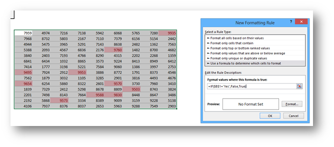
Now here we will do a rule based on the value of the Data Validation Dropdown in cell B1 as visible on the first picture in this post. We will now create a conditional formatting rule based on a formula. We will do this like this. !!First we select the same range of cells as we did for the first rule!!. Then we select Home/Conditional Formatting/New Rule…

…and in the dialog box we will write
=IF($B$1=”Yes”,False,True)
In the “Format values where this formula is true:” input box and set no specific format at the bottom. It’s important that we set no specific format, since this rule will only work as a switch.
Getting the settings right
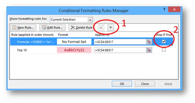
Now this has created the second rule for us, but at this point it has no effect on the previous rules. To achieve this, we must go to Home/Conditional Formatting/Manage Rules… In the dialog box we get, there are two sections demanding our attention. You can see them outlined and numbered in the following picture.
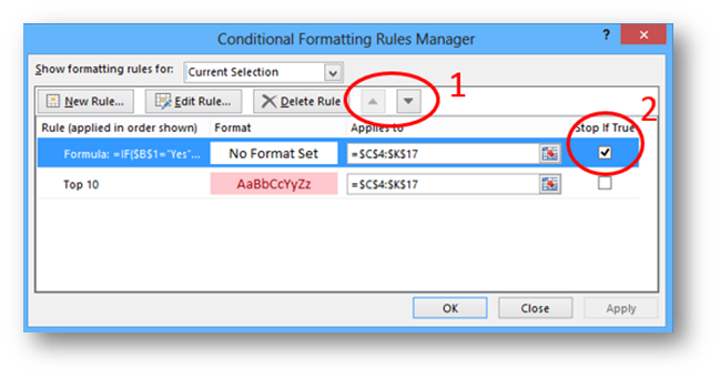
Our first goal is for the Formula rule, to be the first of the bunch… You can achieve this by selecting it and clicking the up-arrow button in section marked with 1. As for the second goal, this will be the magic one. You check the Stop If True Checkbox. And this checkbox says, if the first rule gives true (in other words, if we select “No” from the dropdown in B2), then no other rule will be checked and applied. This also explains, that there can be many more rules bellow, and they all would not be applied in quite the same manner. This truly is a big step to eternal happiness!
Learn more
Check out our YouTube channel and subscribe for more amazing Excel tricks!
Follow us on LinkedIn.
Check out our brand new R Academy!
Related Posts
- November 2, 2021
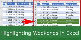
Highlighting Weekends can be hard in Excel. So just for fun, ...

- February 20, 2018
Ever wondered if your could use conditional colouring on Excel ...

- January 16, 2018
This is a follow up post on the final result of last week’s ...
Excel Unplugged acknowledgements


Donate
