Another example how to utilize dynamic capabilities of Power Query comes from our reader. The following post was written as the reply to a great question Dane asked in the Comments section of the Power Query’s Unpivot Function post I wrote back in August 2014. So the question goes like this:

Hello – how do you account for new columns of data being added when using the

1.Change “Null” into 0 step?.

I’ve found that replace values does not pick up new columns when added to the table, thus the unpivot removes rows with null values. How can I make the replace values dynamic as new columns are added?

To simplify, the main part of the question is: “How can I make the replace values dynamic as new columns are added.”

First let’s illustrate the problem with an example. We will start off with a simple Pivot Table.

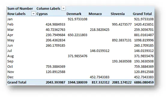
Next we create a Query that takes The Pivot Table and unpivot’s the country columns. So we go from this

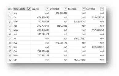
to this

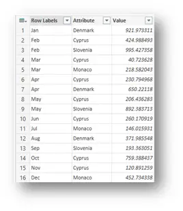
You should notice that the Unpivot command in Power Query simply omits the value “null”. So those “cells” are not represented in the final result. And to “force” them in, what you can do is to do a Replace Values and replace the “null” value with a value of your choice.

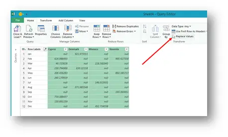
In this case, we’ll replace it by 0 (there are many cases where this would not be the best idea, but let’s just go with the flow for now)

And if we follow up with the Unpivot command

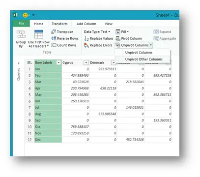
, the result is very different now.

The last step

Now the only thing that stands in the way of this being a fully dynamic solution is the Replace Values step which looking at the code behind the query looks like this

#”Replaced Value” = Table.ReplaceValue(#”Filtered Rows”,null,0,Replacer.ReplaceValue,{“Cyprus”, “Denmark”, “Monaco”, “Slovenia”}),

So the columns, where the replacement will take place, are hard-coded into the line, and if we get additional columns in our Pivot Table, they will not be included in this step and therefore the “null” values will not “survive” the unpivot command. We somehow need to make the (at this point) hard-coded list of columns where the Replacement of values will transpire dynamic. So let’s get to it.

Make it fully dynamic

To start with you need to find the step in your query where the names of the columns are ready for the unpivot command. So I’ll go to the step, where we removed the Grand Total column since we had no intention to unpivot it.

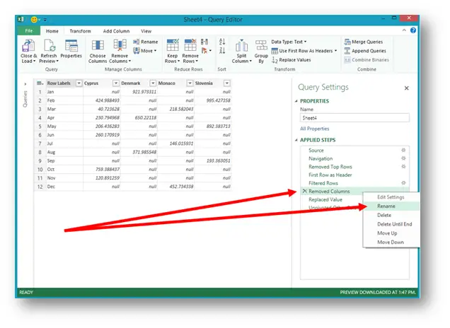
Just to make things easier, we’ll rename that step (Right Click and choose Rename) to Base. And before we proceed, we must make sure, we have the formula bar visible. You can do that by going to the View Tab and choosing Formula Bar.

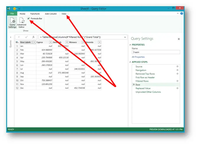
Insert the custom step

Now we press the fx icon and insert a new step that we write manually. At this point you should be prompted, if you really want to insert a step, just choose Insert. Then you write the following fomula in the Formula Bar.

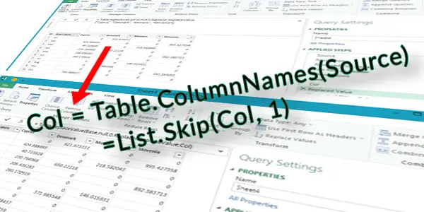
= Table.ColumnNames(Base)

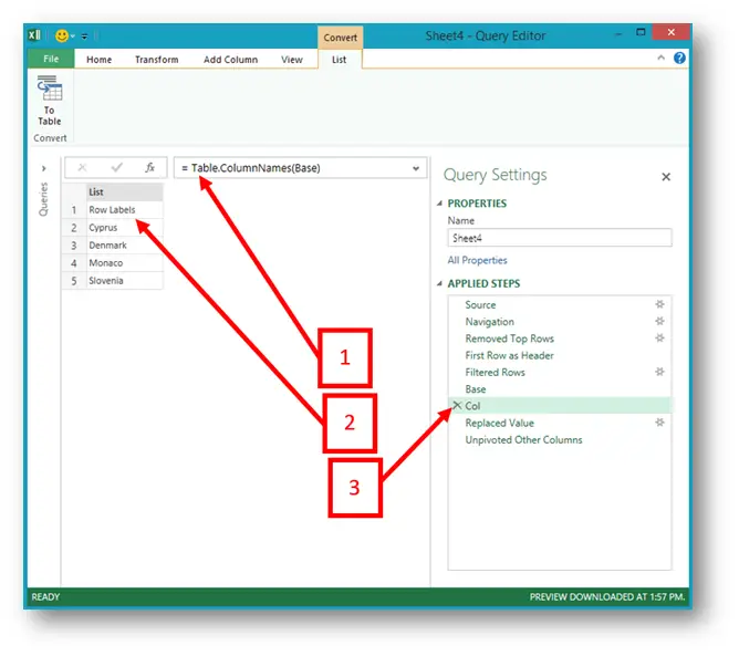
1. After you write the formula just press the check icon and you will create a new custom step
2. Here’s what you get… A dynamic list of all your columns. And the key here is the word dynamic!
3. Next you rename this new step (same as in the previous step) and call it Col. This gives a name to your list, so you can use it in later formulas. (You can leave this step out, but then you should remember the name that Power Query gave to it automatically.)

Now all that’s left to do is to replace the hard-coded list of columns in the Replace Values step with the dynamic list of columns that we just created. Also, we need to change the name of the input step from Col to Base (you should adjust these names to your sample if you weren’t following the steps in full)

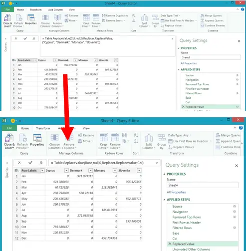
So from

= Table.ReplaceValue(Col,null,0,Replacer.ReplaceValue,{“Cyprus”, “Denmark”, “Monaco”, “Slovenia”})

to

= Table.ReplaceValue(Base,null,0,Replacer.ReplaceValue,Col)

This will replace the “null” values with 0 in all the columns. If we wanted to, we could take this a step further and replace the last bit with

List.Skip(Col, 1)

All this does is it returns the list of all columns but leaving out the name of the first column… With this our formula would look like this

= Table.ReplaceValue(Base,null,0,Replacer.ReplaceValue,List.Skip(Col, 1))

Same principle could be applied to the Unpivot command but that would be much easier to do with selecting the firs column and then choosing the Unpivot Other Columns command. Since this makes our Query dynamic, it brings us one step closer to eternal happiness.

Learn more

Check out our YouTube channel and subscribe for more amazing Excel tricks!

Follow us on LinkedIn.

Check out our brand new R Academy!