Removing old Row and Column Items from the Pivot Table
Pivot tables still remains the go to solution in Excel for Data Analysis. And for those who do work with them on a regular basis, three things begin to bother them soon. One is the automatic resizing of columns on Pivot Table refresh which you can read about here. The second is, that If you use the same data set to create many Pivot Tables, they are all connected to the same Data Cache and therefor all update at the same time, all use the same grouping on lables and so on. If you want to know how to resolve this, you can read about it here. This article will address the third issue with the Pivot Table command that enables you to still see the leftover entries that no longer exist in the data table. We will also talk about how to remove them…
Here is an Example of what I’m talking about. Let’s say we have the following data table in Excel.
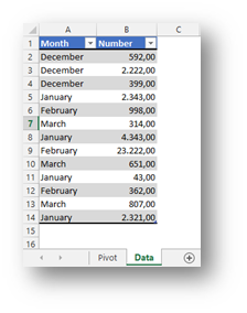
Notice that in the Month column, there are Four Months present, December, January, February and March. Now based on this data, we create a Pivot table where we calculate the Average number per Month.
Nothing out of the ordinary there. Now let’s change the data a bit. What we will do is delete all the December data, as we no longer need it, and add the data for April. So now the data table we are working on looks like this

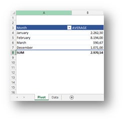
Now after refreshing the Pivot Table, we get something like this

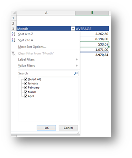
Now that seems perfectly fine, but let us see what we get in the dropdown menu at Row Labels or Month…
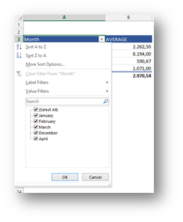
And there it is, although our data no longer has any Rows of Data belonging to December, the December is still part of the Month field as you can see. The record was not deleted from the data model. Now this has some great uses, for example with the GetPivotData function etc. But for the puropse of this article we will discuss how to get rid of the discarded data in two ways. Manually and using a VBA code or a Macro.
Getting rid of old Row and Column Labels from the Pivot Table manually
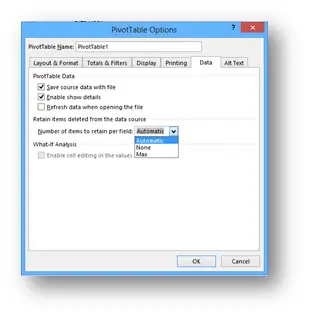
You place yourself in the PivotTable and either Right Click and select PivotTable Options or go to the Analyze (Excel 2013) or Options (Excel 2007 and 2010) Tab. In the PivotTable Options dialog box you place yourself on the Data tab.

The command we are looking for is Number of items to retain per field. The value is set to Automatic by Default and that means that Excel will decide how many items to retain. What we need to do is to change the Number of items to retain per field setting to None and then Refresh the PivotTable. You have to refresh the Pivot Table to see the result!
After doing so, you can clearly see that December has disappeared from the Month field.
Getting rid of old Row and Column Labels from the PivotTable by VBA
If you have more Pivot Tables in a Workbook and you want to do this faster (set the Number of items to retain per field for all Pivot Tables to None) than the option above, you can use the following VBA code…
 Sub DeleteOldPivotData()

Dim PivTbl As PivotTable
Dim ws As Worksheet

    For Each ws In ActiveWorkbook.Worksheets
        For Each PivTbl In ws.PivotTables
            PivTbl.PivotCache.MissingItemsLimit = xlMissingItemsNone
            PivTbl.PivotCache.Refresh
        Next PivTbl
    Next ws
End Sub
And we are one step closer to eternal happiness 🙂
Related Posts
- September 30, 2014
If some pictures are hard to view, you can get the PDF of the ...

- September 23, 2014
We have a dish where I come from (Slovenia), called Minestrone. ...
- August 19, 2014
One might think that analyzing data with a Pivot table is hard, ...

- May 16, 2014
This question or rather comparison never seizes to amaze me, ...
Excel Unplugged acknowledgements


Donate
