How to get the top 10 values in a table, and an aggregate for all the other data? Our goal today is to turn a table of countries with attributes into a table of ten most populated countries plus an additional row containing an average for all other countries.

Utilizing Power Query Lists 2/3

This article is part 2 of the Using Power Query lists series. In this series, we will look at how we can use lists to do the following:

1. Dynamic Filtering on a Column Using Lists
2. Changing a Table of Attributes and Values to retain only Top 10 Attributes (by values) and turns the rest to Others (This post)
3. Dynamically retaining only columns that contain Actual amounts from a Table

We will be using the same Workbook as in the first article. You can get the Workbook here and follow along.

The goal

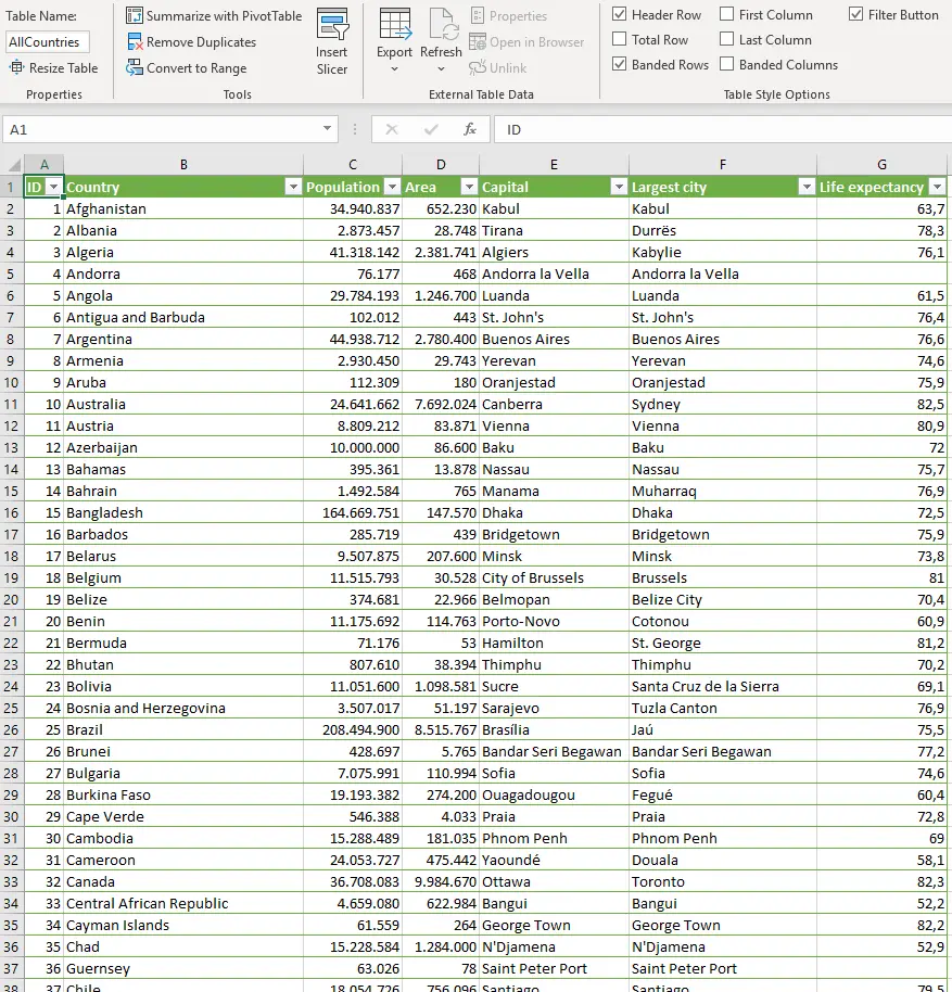
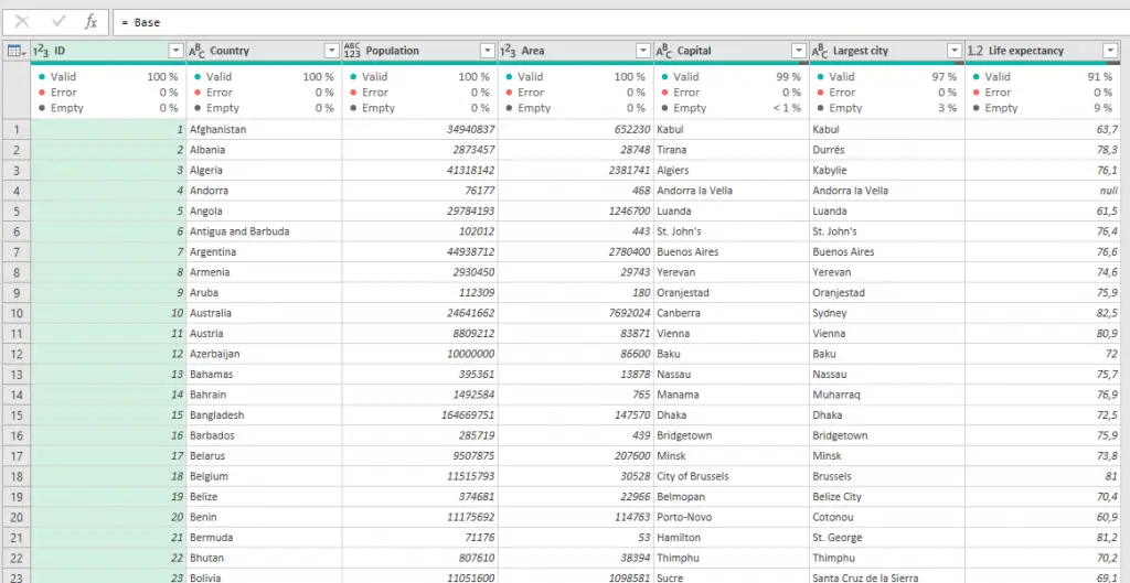
Whereas this is the same Workbookthat we used for the first article and has two tables, we will only be using the AllCountries Table. It contains a list of Countries plus some demographic data and looks like this.

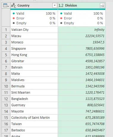
Again, our goal is to turn this Table into a Table of ten most densely populated countries plus a row containing an average population density of all other countries.

We are trying to get this

This is taking things a bit far from the usual use of TOP 10 plus Others where you use simple additions on columns that are already present, but the real brilliance of this lies in the fact that we will achieve everything (including calculations, joins, and appends) within a single query using the dynamic filtering and a few other tricks.

How to: get the data

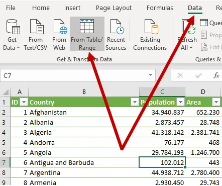
Firstly, we start by adding the AllCountries Table to Power Query by selecting any cell within the Table and using the Data > From Table / Range command.

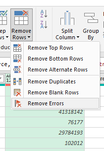
Remove errors

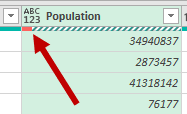
Once you get the data into Power Query you might notice (if you have one of the latest versions of Power Query) that there are Errors in the Population column. This is due to the fact that there is a string (#FIELD!) in that column.

To remove this row, we select the Population column…

…and use the Home > Remove Rows > Remove Errors Command.

Rename the last step

Now that we have a “clean” dataset, we can rename the last step so that we can recall it during the later steps. It’s always a good idea to rename steps from the practical standpoint of better describing what they do, but here there is another reason we are renaming the step. If you want to reference previous steps later in the query, and the step name contains spaces, you have to ad the # sign and double quotes (“”) around the Step name, making the whole syntax needlessly complicated. Therefore it is just good practice to rename steps that you want to reference later so that the names don’t contain spaces.

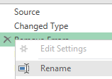
You rename the step by right-clicking it in the Applied Steps window and selecting the Rename Command. We rename it to Base.

Calculate population density

As we want the TOP 10 countries by population density, we need to add a calculated column where we divide the Population column by the Area column. You could do this as a Custom column, but I much rather just use the built-in Add Column > Standard > Divide Command. Be careful to select the two columns in the right order before using this Command!

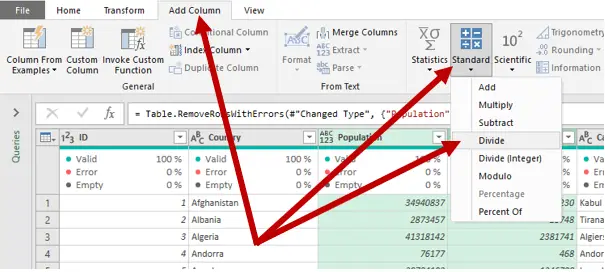
The last step gives us a new column called Division. There is no need to rename this column as it will not be seen anywhere within our final solution.

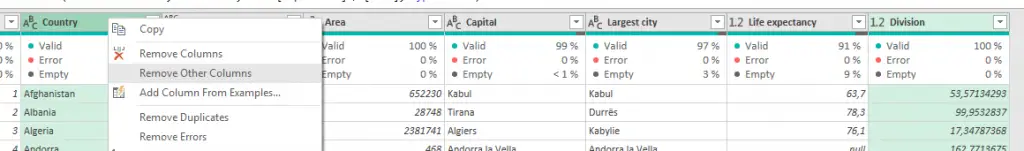
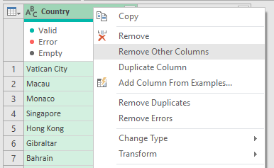
Remove other columns

The next steps are all about getting to the List of the TOP 10 Countries by Population Density. To achieve this, we only need two columns, the Country name and the Division column we just created. We select the two (the order of selection is important as this is the order in which they will be sorted in the newly derived Table) and choosing the Remove Other Columns Command from the right-click menu.

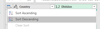
The easiest way to get the TOP 10 list is to sort the data by the Division column. We will sort it with a Sort Descending Command in the Filter menu..

Now we also see there really are miracles happening in Vatican City 😊

Rename

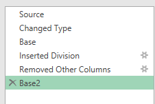
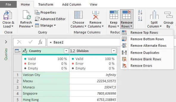
As we will use the result of the last step twice (to get the TOP 10 and to get the Others, we should rename it just as we did with the Remove Errors step when we renamed it to Base. We rename it to Base2 (no spaces, remember ?!?).

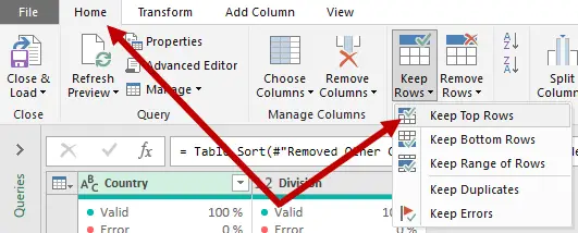
Keep top rows

First, we would like to get the List of TOP 10 Countries. As those are the ones in the first ten rows, we just need to retain only those rows. We do that by using Home > Keep Rows > Keep Top Rows Command shockingly using 10 as the Number of Rows to Keep.

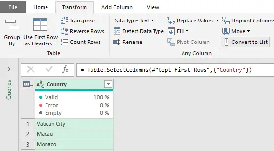
As we just need the List of Countries, we remove all other Columns by choosing the Remove Other Columns from the Right-Click menu.

Create a list

Now we create a list using Transform > Convert to List.

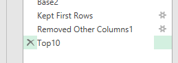
As we will need the List later down the line, we should rename it. You should think of this as assigning the List to a Variable. Let’s call it Top10.

Creating the Others Step

Phase two is where we calculate the Average Population Density of all but Top 10 Countries. First, we need to call back Step Base2. We do this by creating a new blank step by clicking the fx icon in the formula bar and typing a simple formula

= Base2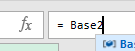

Because we need all but the top ten rows, we will remove those with the Home > Remove Rows > Remove Top Rows Command again using 10 as the Number of Rows to Remove.

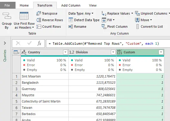
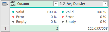
Because we want a single Average, we need to add a Custom Column where each row gets a value of 1.

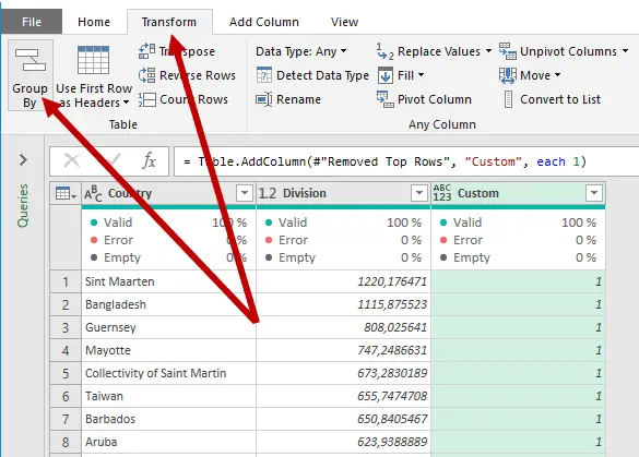
Now we can use the Transform > Group By Command.

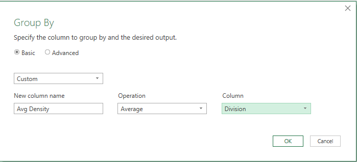
We Group by Custom (which is our column of 1’s and create a column Avg Density by using Operation Average on Column Division.

As a result we get.

Now we need to do three things. Rename the Column Custom to Country, Change that column type to Text and then Replace Value 1 with Others leaving us with this:

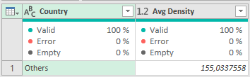
You should rename the last Step to Others.

Putting it all together

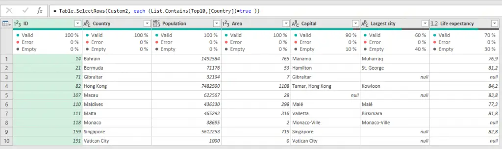
At this point, we are three Query steps away from the desired result, and step number one will be the easiest of them all. Just as before (using the fx button of the Formula Bar), we create a new custom step calling back the Base Step. Power Query calls this step Custom2 (this is important, so check it!).

Step two is two use what we learned in part one of this three-part series of posts to create a Filter step using two previous steps. Custom2, which is our Base Table and the Top10 Step, which contains the List of Top ten Countries. This Step will dynamically filter the Table to only those ten Countries in the List.

Here is the code for the step.

= Table.SelectRows(Custom2, each (List.Contains(Top10,[Country])=true ))

You can get halfway there by simply using the Filter in column Country and then just change the rest (like we did in Part 1) or start with a custom step again. Either way, you should end up with something like this:

Finally, all that is left to do is to combine this with the step we called Others. Don’t worry about the fact that the Others step has only one column in common with our last step and even has an extra column that is not even present in our original Table. Power Query was built to handle situations like this 😊. In this final step, we will be simulating an Append Queries action but with two steps of our query. We start by using the fx button one last time and use this code:

=  Table.Combine({#"Filtered Rows", Other})

A simple Table.Combine function on steps #”Filtered Rows” and Other and voila:

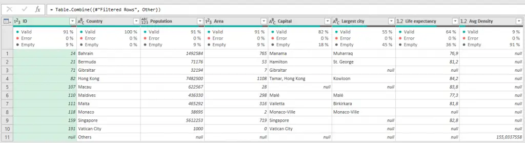
And whereas it is not a beauty to look at, the brilliance of the method itself is amazing.

You can download the Workbook with the final Query here.

Is the next part of this series, we will be using lists to keep only columns with Actual data.

Learn more

Check out our YouTube channel and subscribe for more amazing Excel tricks!

Follow us on LinkedIn.

Check out our brand new R Academy!