Join Types in Power Query – Part 1: Join Types

Who doesn’t love Join? It’s like Excel’s LOOKUP, but better! I use Join all the time for merging tables one way or the other. Let’s look at all the different Join types in Power Query. And then we’ll take things further in Part 2: we’ll create a LOOKUP Dashboard, which will be a single table, but also a concept you can develop onwards.
Join Types
What are all the possible join types? We’ll look at the following:
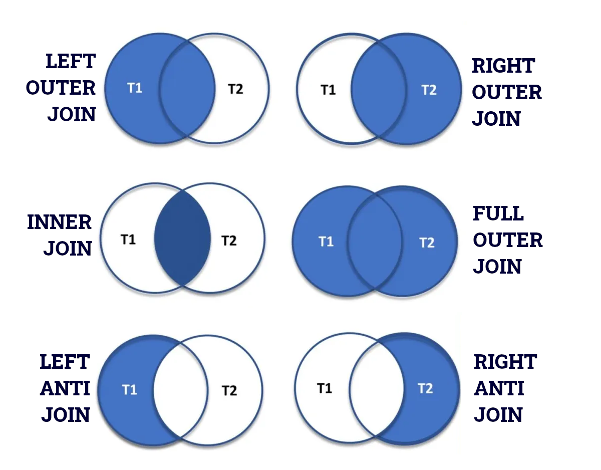
- Left Outer Join
- Right Outer Join
- Full Outer Join
- Inner Join
- Left Anti Join
- Right Anti Join
So if we represent left and right table T1 and T2 graphically, joins would look unions on the image below.
Let’s look at how this looks like on actual examples.
Starting data
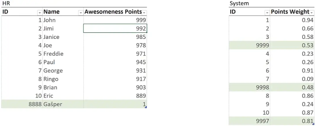
Our data will consist of two tables called HR and System. You can find the file I used here.
Tables contain records that can be matched up based on the common ID column. We also have a few records that can’t be matched up. We highlighted those records with green.
We bring both tables to Power Query with selecting a cell in the table and then selecting From Table/Range.
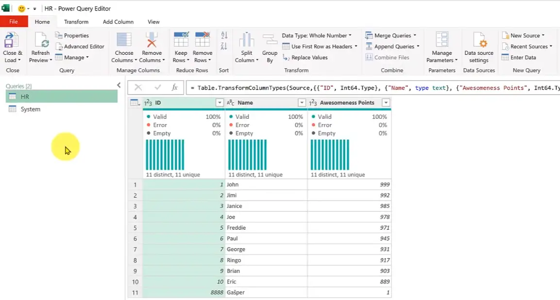
Now that we have both tables in Power Query we can start exploring Join types.
Left Outer Join
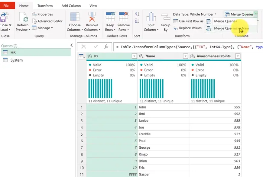
Let’s select the first query called HR and then Merge Queries > Merge As New.
Merge dialog shows up. Select the HR table as the first table and the System table as the second.
Set Join Kind to Left Outer (all from first, matching from second).
Select ID column in both tables as the common column. The name of the common column doesn’t matter, but the type does – it has to be the same.
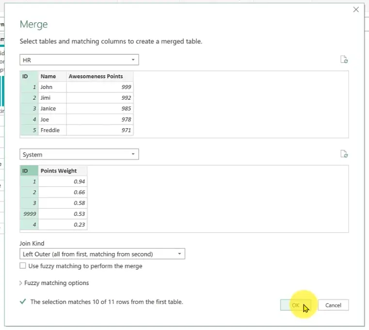
Confirm with OK.
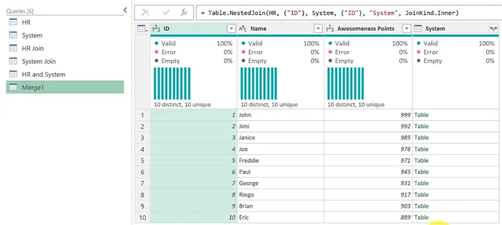
We get the following result.
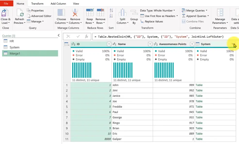
Select the Expand icon (two arrows) on the System column.
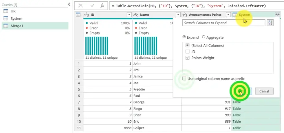
Select only Points Weight column and remove the tick from Use original column name as prefix option.
Confirm with OK.
We get the merged result!
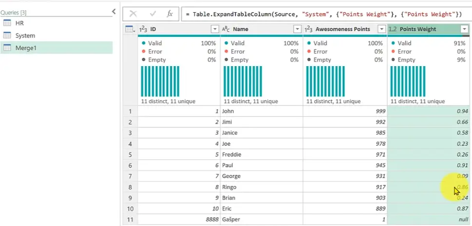
We can now see the record that wasn’t found – the last one.
For clarity we’ll rename this query to HR Join.
Right Outer Join
Now repeat the process, but this time select Right Outer (all from second, matching from first) Join in the Merge dialog.
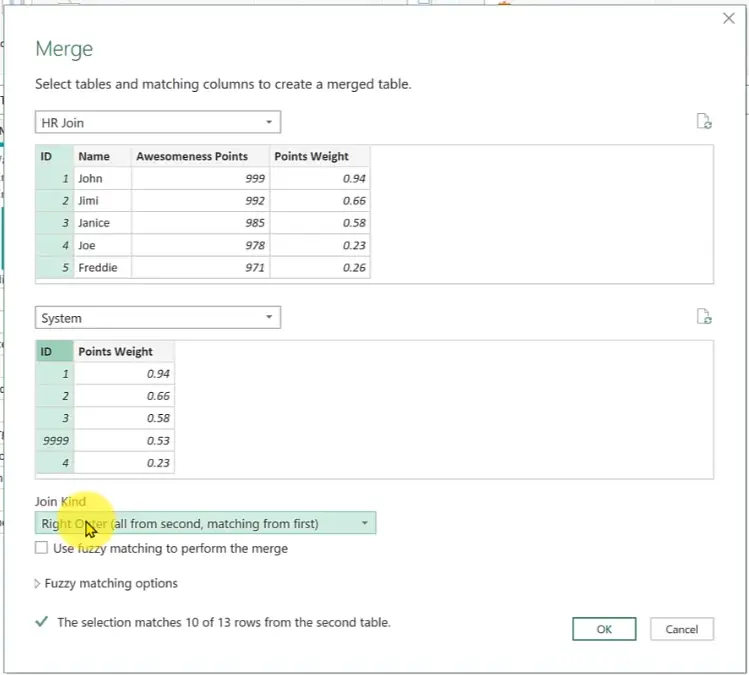
We get the following result.
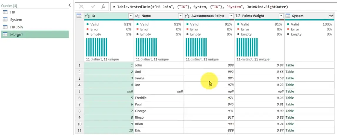
Again select the Expand icon on the System column.
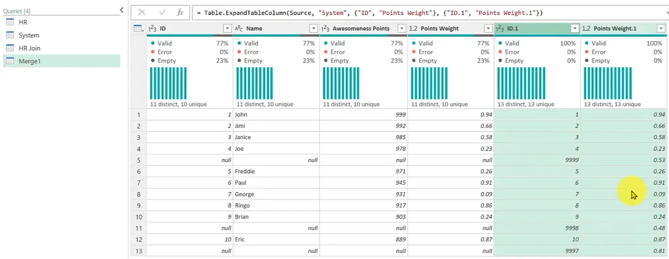
We got all the records from the second table, but only the matching one from first. It maybe a bit counterintuitive view, so let’s move the last two columns to the left.
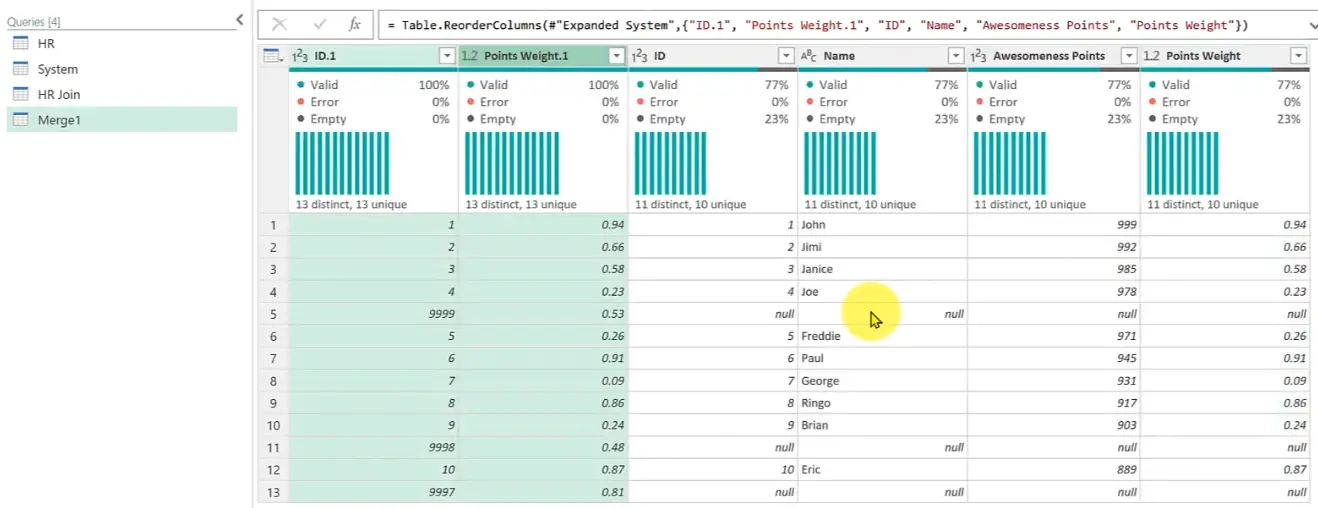
Voila, another useful view!
Rename query to System Join.
Full Outer Join
What about if we want to know everything, match or not? We use full outer join!
Repeat the process again, but select Full Outer (all rows from both) in the Merge dialog.
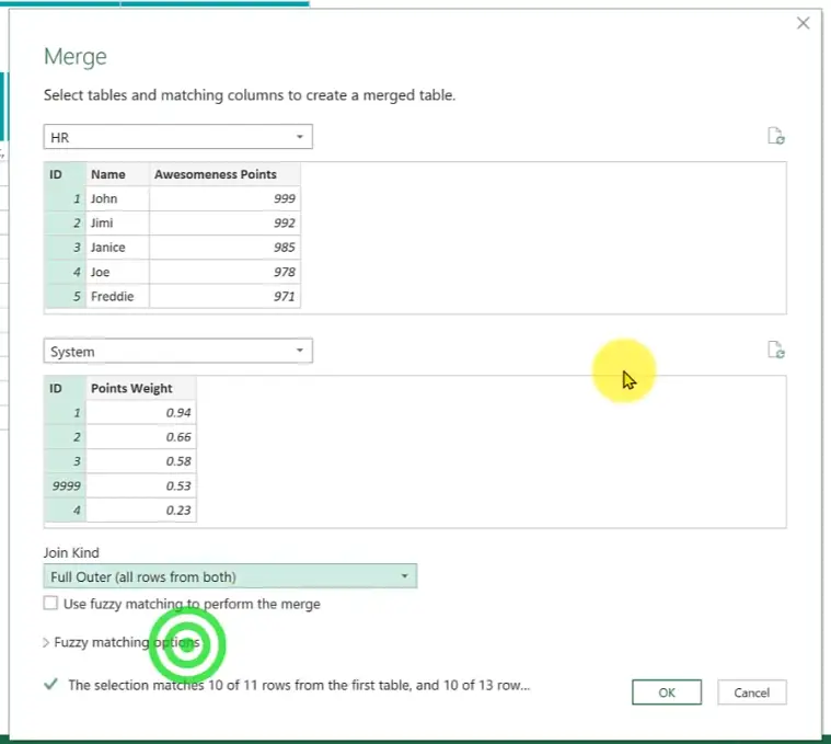
Confirm with OK.
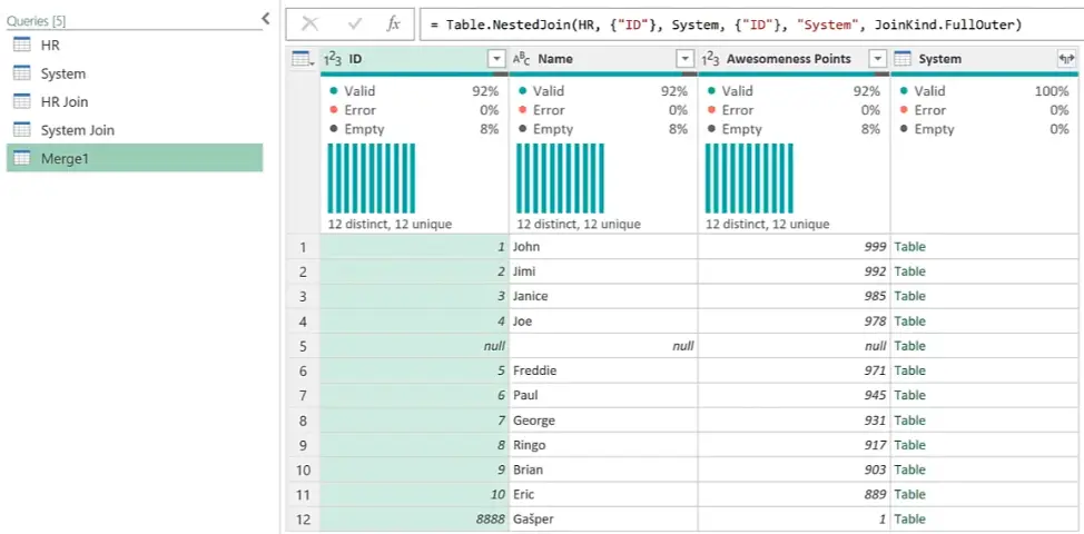
Again use the Expand on the System column.
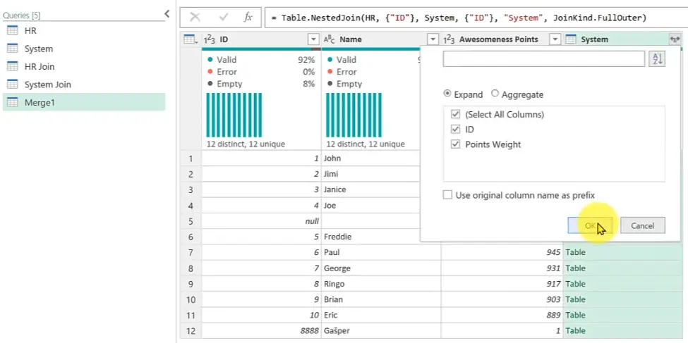
Select both columns and confirm with OK.
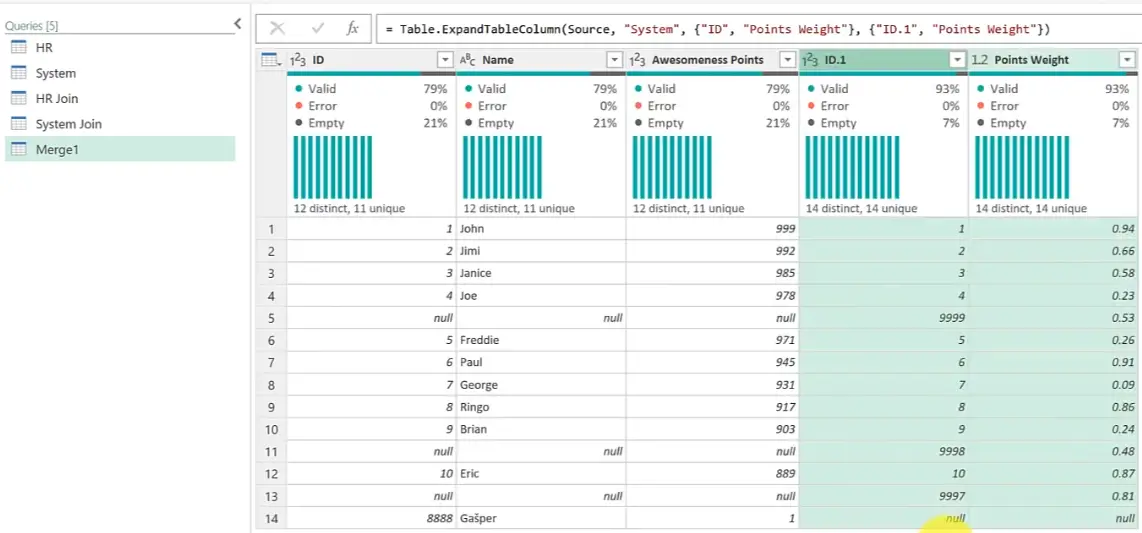
We see all the records, matched or not!
Rename query to HR and System.
Inner Join
Let’s go the other way now, we would only like to see the columns that match up. We select Inner (only matching rows) in the Merge dialog.
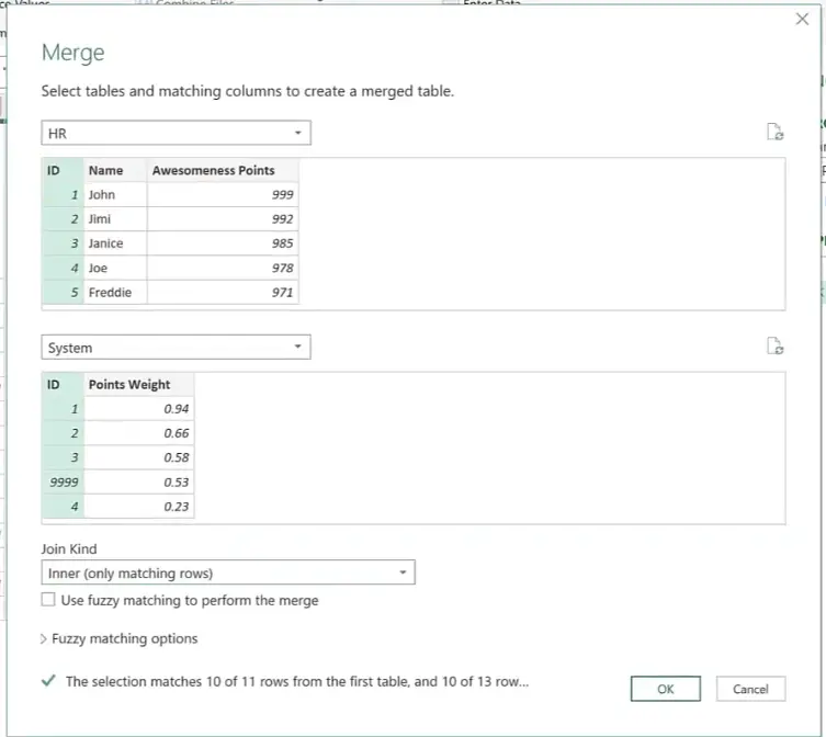
Confirm with OK. We get the following result.
Use Expand to bring in extra columns.
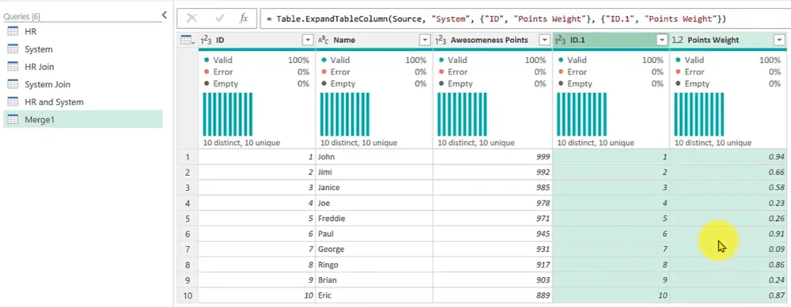
We get only the matching records from both tables!
Rename query to Inner.
Left Anti Join
Now we’d like to see everything from HR that couldn’t be matched to the System table.
In the Merge dialog, select the Left Anti (rows only in first).
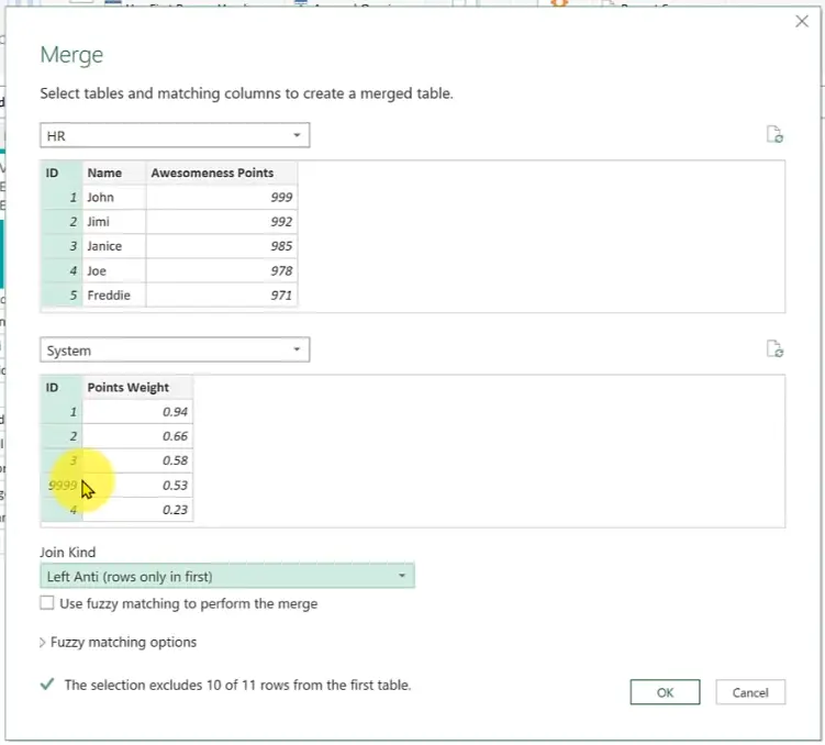
Confirm with OK.
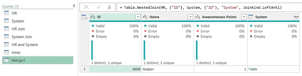
As expected we get only one row. We can delete the last column.
Rename query to HR only.
Right Anti Join
Similarly, let’s get everything from System table that couldn’t be matched to the HR table.
In the Merge dialog, select the Right Anti (rows only in second).
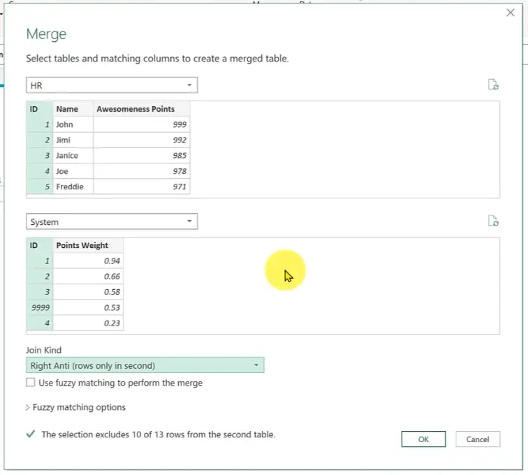
Confirm with OK.
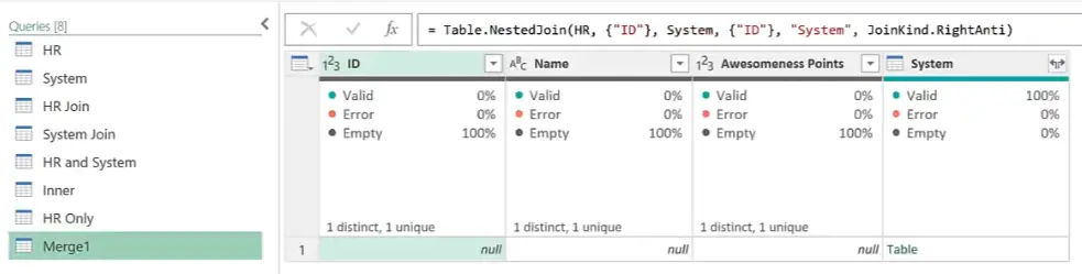
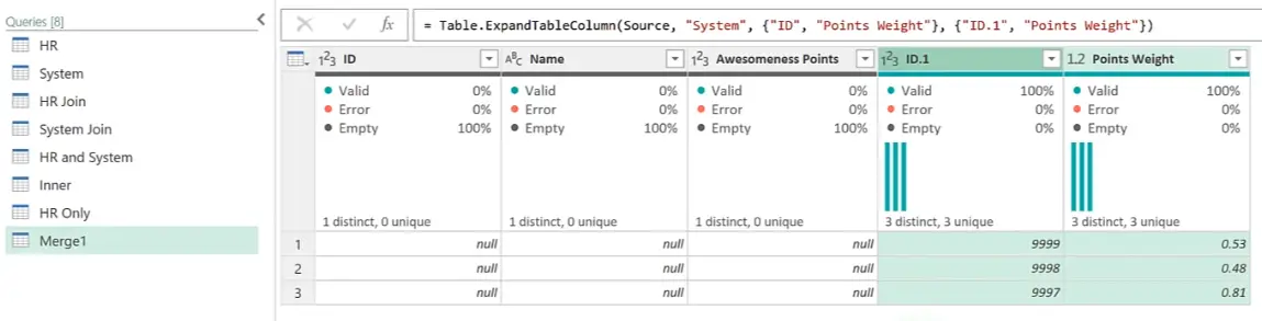
Expand the System column.
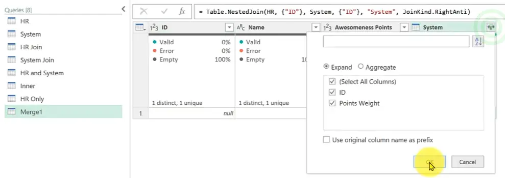
We get the actual content on the right, which might be a bit counterintuitive.
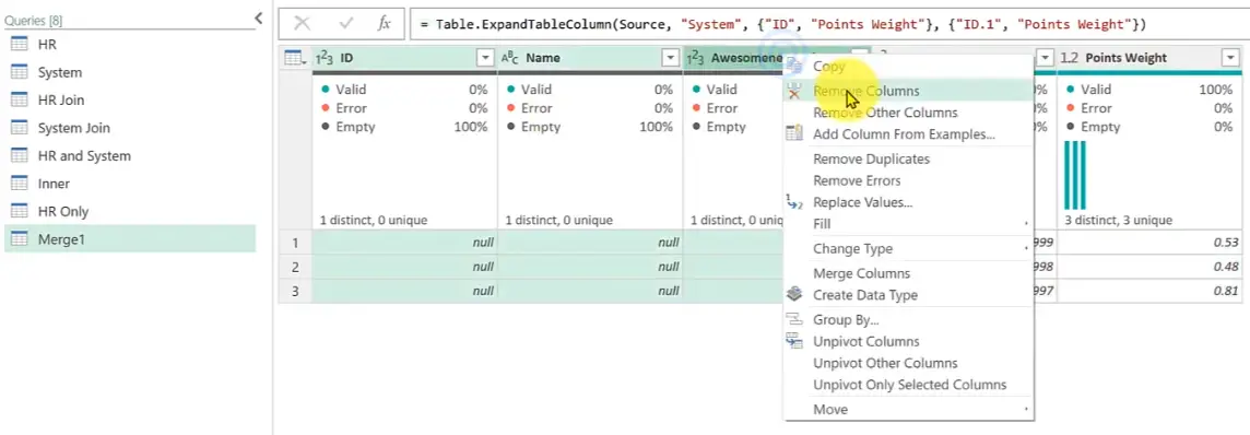
Let’s just remove the first three columns.
Voila! Here’s our answer.
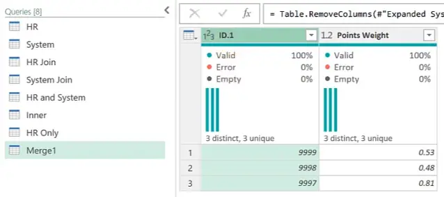
How simple was that?
We were able to get all kinds of information from different join types. We’ll now take things further: stay tuned for Part 2, where we’ll create a LOOKUP Dashboard, which will be a single table, but also a concept you can develop further!
Watch the tutorial
Meanwhile, you can also watch the tutorial online on our YouTube channel!
Please leave us a like, comment, and subscribe for more amazing Excel tricks!
Follow us on LinkedIn.
Check out R Academy!
Excel Unplugged acknowledgements


Donate
