Formula to get quarters from dates in Excel

We have a column of dates in Excel, and our goal is to get Q1, Q2,… or QTR1, QTR2,… or Quarter 1, Quarter 2,… . I think you get the picture 🙂
First we will show the simple formula to get quarter number from dates. Then we will show how to add any prefix to that (like Q, QTR or Quarter…), and then we will show how to modify your formula starting with any other month. Let’s say July 1st is the beginning of Q1. Let’s dive into it.
Getting quarter number from dates
You actually get the quarter number from month number which you extract from the date. There are two basic ways to do this, presuming the date is in cell A1
=ROUNDUP(MONTH(A1)/3,0)
=INT((MONTH(A1)-1)/3)+1
As you can see the differences are purely cosmetically but they both give you a quarter number. If you already have a month number in a column, you can replace MONTH(A1) with a reference to the cell with the month number.
Adding a string in front of the quarter number
Now to add a string like Q, QTR or Quarter in front of the number
= “Q”&ROUNDUP(MONTH(A1)/3,0)
= “Q”& INT((MONTH(A1)-1)/3)+1
So you add the string or better yet the prefix you want in front of the previous formula, dress it up in apostrophes (“) and add a ampersand (&) to append the number to the string. If you want the result to be Quarter 1, the formula would be = “Quarter “&ROUNDUP(MONTH(A1)/3,0). You may notice an extra space after the Quarter but inside the apostrophes, which is purely cosmetic.
Starting Q1 with any month you want
Now this is where it gets tricky, but it is done with one general formula. First the formula (this is a formula that will start Q1 with July)…
=ROUNDUP(MOD(MONTH(A1)+5.1,12)/3,0)
There are three new things here, and they will be explained individually, but first, the value that determines which month will be the first month of Q1. In our case it’s 5.1 because we want to start with July. Here is a table of values to use in the formula (the rest of the formula stays the same) with corresponding starting months.
|
January |
February |
March |
April |
May |
June |
July |
August |
September |
October |
November |
December |
|
– |
10.1 |
9.1 |
8.1 |
7.1 |
6.1 |
5.1 |
4.1 |
3.1 |
2.1 |
1.1 |
0.1 |
Now for the rest of the formula. You take the month number and add a value to that. If the value is 7.1 (so may is the first month of Q1), and you take a date that starts in November, you will get 11 + 7.1. This will give you 18.1 and as for the month numbers, the 18th month is unheard of, so we will use the MOD(number,devisor) function, where the devisor will be 12. This means that 18.1 will actually be 6.1 after the MOD function gets through it. As you divide this by 3 you will get 2.033333 and after the ROUNDUP function is done, this will be 3, so November is in Q3 if May is the start of Q1 which is correct.
Hope this article was helpful and it got you closer to eternal happiness :). I recently wrote about another way to get quarter from dates. Zou can read about it here.
Related Posts

- October 5, 2018
One of the most popular posts on Excel Unplugged is Formula to ...

- February 24, 2015
Surprisingly, this is not a post about the Translate feature in ...
- April 16, 2013
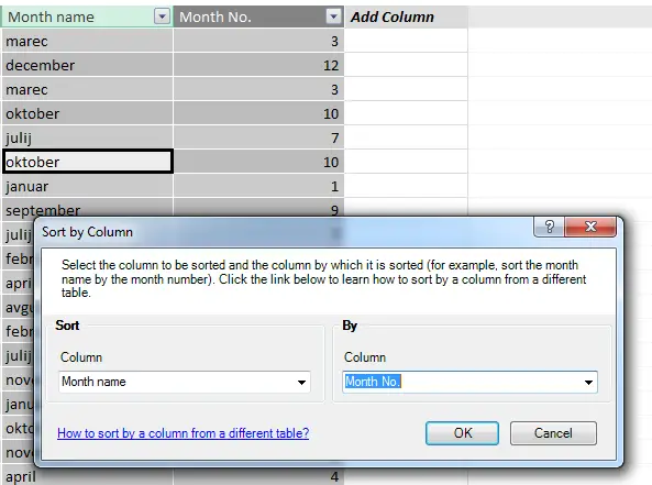
Here is our “problem”. When you create a Pivot Table ...
Excel Unplugged acknowledgements


Donate
