Excel has quite a few funny perks. Once you get over the 15 digit limit in Excel and the fact it does not calculate exactly as it should, you will sooner or later arrive at the point where you will feel the need to calculate time. In this case time stands for time and date formats in Excel. This is where things can get really strange. First we will look at dates and then hours.

Dates

01/01/1900 or 01/01/1904

The two dates are actually two modes in which Excel can deal with time. In the first mode (01/01/1900), which is also a default mode on a Windows computer, Excel starts counting the days from 01/01/1900. That day has number 1 behind it. And every other date has a number behind it also. For example, 04/13/1948 has 17 636 behind it. That only tells us, that 04/13/1948 was 17 636^th day after 01/01/1900. But on Apple computers, the first date by default is 01/01/1904. So number 1 means 01/01/1904. Now imagine you are sending a file that has 01/02/1900 in a cell. All that Excel knows about that cell, is that the value of a cell is 2 and the format is Date. So when someone on a Mac will open it, he will get…

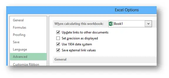
You guessed it, 2.1.1904. And this four year leap is repeated across all dates in your workbook. Another reason, 1.1.1900 might not have been the best idea to start with, is the 02/29/1900, which will be covered in the “Feb 29^th 1900 was a Wednesday” section. Now to overcome all this or better yet to switch between the 01/01/1900 and 01/01/1904 modes you can go to FILE/OPTIONS/Advanced and then in the “When calculating this workbook:” section you select the “Use 1904 date system”.

Feb 29^th 1900 was a Wednesday

In this case Lotus is to blame and not Microsoft. They only adopted the solution (it would be better said adopted a problem, but as John Lennon says “There’s no problems, only solutions”). But the problem is there nonetheless. So what is the problem? Well, 02/29/1900 in reality did not exist, but in Excel (using the 01/01/1900 mode) you can write it and even see what day it was J

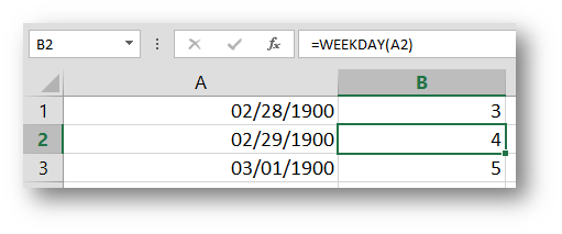
It was obviously WednesdayJ. The problem is, that 02/28/1900 returns Tuesday and 03/01/1900 obviously Thursday, but in reality, they were consecutive days. So if you are looking for a difference in days between 01/01/1900 and 04/13/1948 you will get one day too many, since Excel thinks that 29/02/1900 was day #60 from the 01/01/1900 but in reality 03/01/1900 was.

=DATEDIF()

One more thing that Lotus brought along. The DATEDIF function is very interesting since it officially never existed in Excel (not counting the accidental mention in the help file of Excel 2000). But despite its nonexistence, you can use it to calculate the difference between two dates in Excel.

Basically you do something like =DATEDIF(Date1,Date that occurred after date1,”y”) and you get how many years passed between the two dates. The last argument can be “m” for months, “d” for days or “ym” for the remaining months over the calculated years and “md” for the days over the last calculated month.

For instance, to calculate the difference between 04/13/1948 and 12/31/2000 in years, months and days, one would do

=DATEDIF(04/13/1948,12/31/2000,”y”)&” Years “& DATEDIF(04/13/1948,12/31/2000,”ym”)&” months “&DATEDIF(04/13/1948,12/31/2000,”md”)&” days.”.

Time

Now time in Excel is just a decimal number that can tell you what percentage of the day has already passed.

So adding time should be very easy.

Adding time

Adding time is very natural. Let’s say it’s been a slow week and you only worked 12:23 on Monday, 14:53 on Tuesday and 11:28 on Wednesday. Now you wish to add those up. So you do a SUM of those three values

and you get

The result should be 38:44 but instead we get 14:44. So what’s happening? Well like we said before, time is actually a decimal number for Excel. So in the first three cells we have

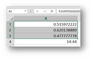
And when we add those values up, we get

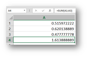
Which is quite logical, but we want to see the result as time, so we change the format and get

Well it’s 14:44 again. Now the value in a cell is 1.6138…, and Excel strictly speaking understands this as 14:44 on 01/01/1900. But if you want for hours to go over 24, you must use the following Custom Format [h]:mm. As you can see in the image bellow, this drastically changes the way we see the output

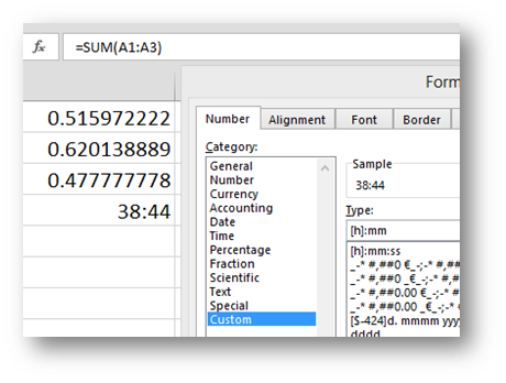
So now we can add time. But how about subtracting time?

Subtracting time

This is an even bigger conundrum. Let’s say we got the following time values and formula.

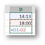
Pretty straightforward right? Here’s the result

You get an endless ####… So how can you subtract time in Excel? Well, remember the 1904mode in Excel? It’s the magic wand in subtracting time!

I’ll leave the formula as is and just switch Excel to the 1904 Date system and Voila

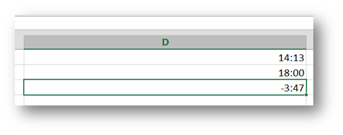
But what if we were subtracting 14:43 – 66:44? Well you’ll still need a 1904 date system but it will give you  -4:01. Now all we need is…

You guessed it [h]:mm Custom Format and you get -52:01.

Eternal happiness 🙂