Sometimes in Excel, people insert data in places where they weren’t supposed to. And even if they remove any trace of their wayward journey, a scroll bar remembers it. I call this Scroll Trouble in Excel. This post will show you how to make Excel “reset” the Scroll Bar in three different ways.
If you like learning from Video more that you do from Blog Posts, here is a link to a video on my YouTube channel teaching you basically the same thing: https://bit.ly/3wOno82
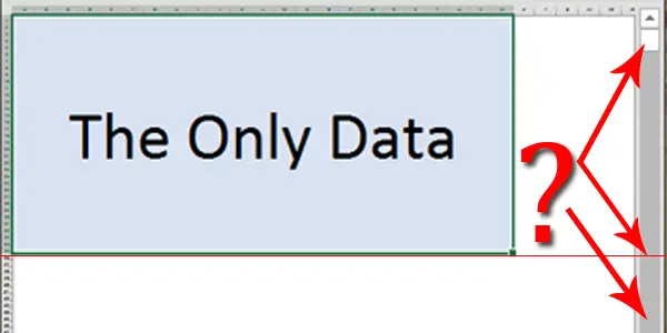
Just for reference, this is what we are talking about.
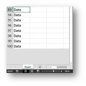
We have Data in Cells A1:A100. At this point the vertical Scroll Bar goes from row 1 to row 100.
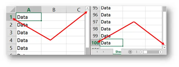
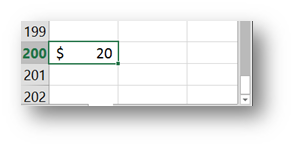
Now someone decides to put something non trivial (something that includes some formatting like a date or currency) into cell A200. And it’s not a shock that at this point, the vertical Scroll Bar goes all the way to row 200. All as it should be so far.
But then you delete this entry and Save the file. One might expect for the scroll bar to go back to row 100 as the bottom line, but it does not. Now we have Scroll Trouble in Excel.
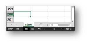
Now here’s a famous saying. This is a feature! Excel thinks that since you have taken the time to format cell A200 that cell must be important to you and you are just waiting to input some data into it and therefore it still gives you the ability to move swiftly to it by using the scroll bar. But our problem is that cell A200 has no value for us and we would like for the scroll bar to only go from the first row to the last row with data (in this case row 100).
Here is how you can get rid of Scroll Trouble in Excel in three different ways.
Whereas this is not an ideal solution, it does provide you with the desired result. What you do is you select all the Rows bellow your data (or Columns to the right of your data, depending on which Scroll Bar you wish to adjust), Right Click and select Hide.
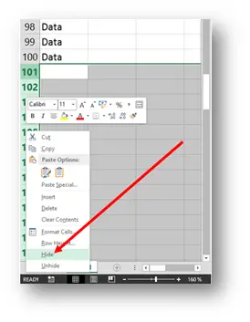
Since this will hide all the rows from the hundredth down, it will therefore adjust the Scroll bar which now does stop at row 100.
But just to be clear, this means that every time you wish to add data, you would have to unhide the rows you need and then add data which can be quite time consuming so in those cases, choose one of the following ways to get a desired result.
Now in this case, we will truly deal with the root of the problem. Removing the invisible data that still resides in cell A200. It’s very important that you understand that Delete key only deletes the cell content, it does not remove the cell format. To do that you must delete that cell! The best way to do that is to select the first row bellow the data and down to the last row. After selecting all the rows that don’t contain data press Ctrl + – (so Control and minus). This will delete those rows and any formatted cells that lurked in the depth bellow the data :). But still the Scroll Bar will remain as it was until you save that file! And right after you do, you get what you want
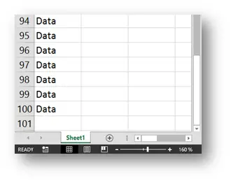
I hope that you noticed a distinction to the previous method where here you still have rows bellow 100 visible and ready to go!
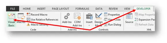
It’s actually two separate methods. The first one only requires you to use the VBA editor. To get there either press Alt + F11 or go to DEVELOPER/Visual Basic
In the VBA Editor window choose the Excel Sheet where the Scroll Bar has stopped cooperating with you and in the Properties Window (if you can’t see it, choose View/Properties Window or press F4) adjust the ScrollArea Property to the desired value (in this sample that is A1:A100 (the dollar signs will be added automatically)).
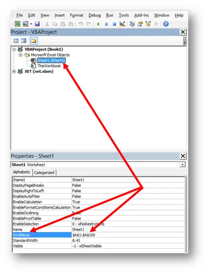
Something very interesting will happen then. The Scroll Bar will not adjust as one might expect but if you try to scroll below row 100, you just can’t :). This can be quite useful in some situations but it is not as elegant and not as useful as Method 2 in this case.
Now the second way of doing this within Method 3 is actually doing the same thing but with VBA code.
Sub SetScrollArea() ActiveSheet.ScrollArea = "a1:a100" End Sub
So this piece of code will do the same as the first sample in Method 3.
Keep in mind, this is also a great way to protect your sheet or data beyond a certain point without actually using Sheet protection.
Here is a video version of this post:
Happy scrolling.
This site uses Akismet to reduce spam. Learn how your comment data is processed.
Instead of deleting the row to remove the formatting, you can simply use the Clear All feature on the ribbon. Select the cell(s) that has/had the data, select the Home tab, in the Editing group, select the drop arrow beside Clear and select Clear All. You will still need to save the file to get the scroll bar it reset.
Hi Larry!
You are right and I also pointed out in the article that deleting the rows is not the best idea. However, Method 2 from the post does exactly what you suggest but far quicker. In effect, clearing those cells will do just the same as Ctrl + – but Ctrl + – is much quicker that going Home/Clear/Clear All. But again, although it’s not the same thing, it has the same effect as Method 2.
this works for me, method 2 takes up some time to delete..just hold ctrl while pressing down and left to select all cells quickly
I have been searching for a solution to this problem all night. Method 1 is not practical for me, and method 2 does not work (though I’ve tried about 100 variations of it at this point). I have a spreadsheet with almost 50,000 active rows, but the scroll bar is taking me down to over a million, so method three doesn’t help the situation much as the shrunken scroll bar still cannot move with any trace of accuracy. Any other ideas?
I have had the same problem….Method 3 would work I assume, but I’d much rather get the desired result from Method 2, which is not cooperating at all so far. Any ideas would be appreciated
Maybe it’s the Ctrl + – combination that’s failing you, try selecting the unused rows bellow the data and select Home/Delete/Delete Sheet Rows
Thanks for this tip. Worked as described!
forgotten to add: Method 2
@John
Nice to hear that John… So now you’re one step closer to eternal happiness 🙂
Nice one Gasper – Method 2 worked a treat, thanks (I never tried the others)….
Thank you. I’ve been looking for a solution to this for a long time.
Big like!
Now for a challenge…. I have a worksheet with 1500+ rows. The row size in height vary greatly.
When I leave the row size alone, the scroll bar is an appropriate size and scrolling to the bottom takes me to my last row.
Once I resize each row to a height of “15”, the scroll bar expands exponentially. This results in the tiniest movement jumping 100’s of rows.
It seems that it represents the original “Volume” that the expanded row used to occupy.
None of the Clear, Delete Rows, and Save tricks work at all.
Excel doesn’t adjust to the new size of the displayed data.
Thoughts?
Hi,
I tried to replay your scenario and it didn’t work as you described so I think It’s a file specific thing. Can you recreate it in a new workbook?
Yes i can create it in a new workbook.
I have many examples of this all with different data.
Now I’m intrigued 🙂 Could you share one with me?
It helped. Thank you.
Thank you.
I have sitting at my desk for hours trying to figure this out.
your Method 2 work easily and perfectly for 2013.
Thanks
I am having a seperate issue entirely, but I can’t find any forums on the matter….
I have a spreadsheet where about 30 rows are hidden for function. But if I wanted to unhide them, I go highlight one row (#35) and drag with finger held on mouse to upper limit row (#5) in preparation of right-clicking ==> unhide. Simple.
But once my mouse reaches the upper limit row excel rapidly scrolls the highlight down to row 165, I have no data beyond 125. Seems random, same problem across multiple computers, and it’s not even happening consistently (~50%).
Any ideas?
Try writting 5:35 in the Name Box and see what that does for you…
Hi, i am currently able to apply scroll lock on running application but it disappears as soon as i close the excel sheet. When reopened same file, scrolling is as free as ever. Is there any way or VBA code that helps implementation of same scroll lock even after closing and reopening the file??
That would help me a lot.
Thank you.
Try method three of this post. Set a ScrollArea for the desired Worksheet. That is a property that will be retained with the workbook.
Thank you so much! This has been driving me crazy! I’ve tried highlighting and deleting cells – but it must not have been a large enough range. The “Ctrl”+”-” saved the day…and my sanity!
so cool! Thank you. I’ve been using Excel since my IBM working days and I had completely forgotten how to do this trick. Thanks for this post (and reminder for me). 🙂
Thank you…! I used method 2, just to add one quick tip, after selecting the first empty row, press CTRL + SHIFT + DOWN ARROW to select all the rows up to infinity and beyond…then press “CTRL and -” and save, and viola! The world makes sense again! 🙂
Thank you much – been struggling with this for years. I used Method 2
Glad to hear it Liz. Not that you’ve been struggling for years but that you will never struggle again 🙂
Look for forgotten OBJECTS! The above solutions won’t delete them. Worked for me.
Thanks a lot!
Your idea helped me!
Glad to hear that!
Saved my sanity!! I used Method 2 and worked just fine after I saved my file. Thank you so much!!
My pleasure Gabriela.