Custom Views or Excel Tables (Sophie’s Choice in Excel)
- Gašper Kamenšek
- March 10, 2015
- 21 Comments
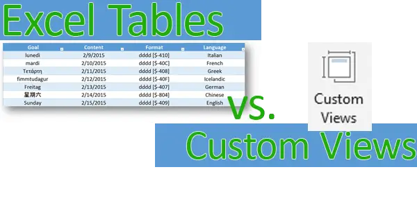
Custom Views or Excel Tables? This is really a lose – lose situation in Excel and therefore a true Sophie’s Choice. Let’s elaborate on the two commands.
Excel Table

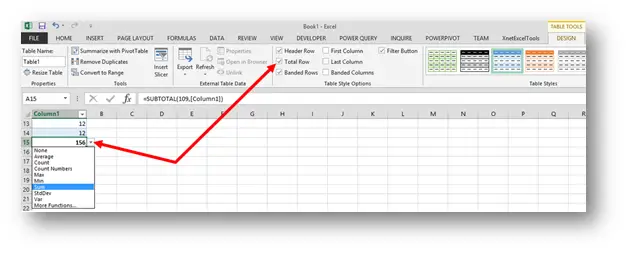
A table is the best way to make Excel dynamic. If you format your range as a table, all your charts that would take data from that table would be dynamic. So you would never have to select the data for a chart when you input new data again. Your formulas also take on a new look. Instead of =SUM(A1:A100) you now have =SUM(Table1[Column1]) and that formula is dynamic. Among other benefits, the Total Row should be mentioned. An aggregation formula can be chosen from the dropdown list and in addition takes into account all your filters. In the picture bellow, you can also see that the title row replaces the Headings of columns. Instead of A you now see a “Column 1” title.
Above are just some of the reasons why you should use Excel Tables in Excel if that is in any way possible, particularly if you want to use Pivot Tables.
Custom Views
Now imagine that a certain Excel file is viewed by many different users, or being used by one user but in many various ways. Now once you need to filter your data by three conditions and sometimes you wish to have six totally different filters applied. Also sometimes you hide a few columns for printing purposes and at different times, you might wish to see all the columns or better yet, hide a different set of columns.
All this can easily be solved by using the so called Custom Views. You can find the command on the VIEW tab.
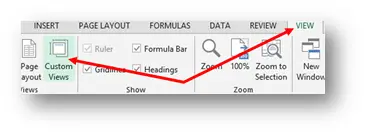
When you use the Custom Views command, you get the Custom View manager. 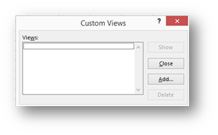
Here you can Show different views or create a new Custom View by choosing the Add button. When you choose to create a new Custom View, you get the Add View window.
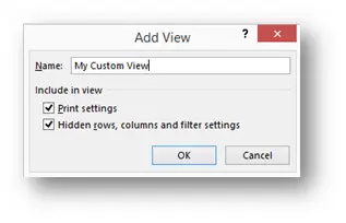
Here you give it a name but more important, here you set if you want this View to remember the current Hidden rows, columns and Filter settings and/or Print settings. If you do save all of them, the next time you want to use them, all you need to do is to regardless of the current view you have of your data, you just choose VIEW/ Custom Views, select the desired view and press Show. All saved settings will be applied instantly. Pure brilliance.
The Choice
But there’s a catch. If you only have one Table in your entire Workbook, you cannot use Custom Views. The command is inactive.
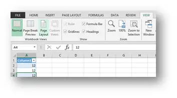
So it really is a Sophie’s Choice. You can only use one or the other but not both. And this goes even deeper. If you use any of the Power BI features, you are almost certain to use Excel Tables and therefore you already know, that you cannot use the Custom Views command. The disappointment is almost as great as the first time you figure out that you cannot use the =Table1[Column1] syntax to define a Data Validation list source. So this really is a great shame and has even gotten me to a point where I installed Visual Studio on my computer, started studying C# and VSTO to try to make it work myself 🙂 . The lengths we go to for a good cause 🙂
Learn more
Check out our YouTube channel and subscribe for more amazing Excel tricks!
Follow us on LinkedIn.
Check out our brand new R Academy!


