Consolidate Multiple Excel Sheets From Multiple Excel Files

We often have our data spread out in multiple Excel workbooks and sheets. How do we combine all of them into one table? Let’s walk through an example.
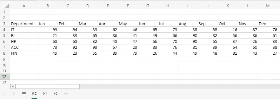
We have our data saved in a folder with three files: 2019.xlsx, 2020.xlsx, and 2021.xlsx. You can download the files here. Each file contains three sheets: AC, PL, and FC.
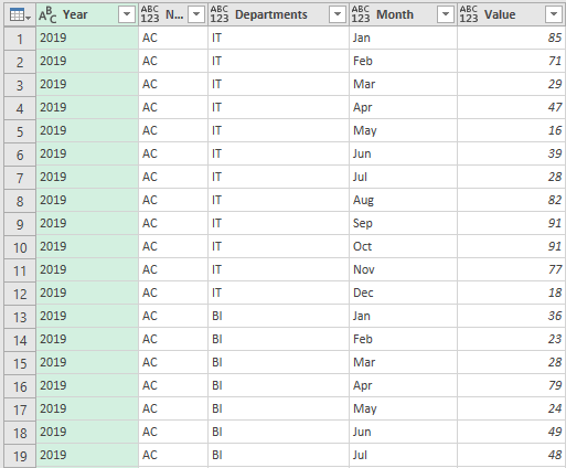
Data from the 2019.xlsx file looks like this:
Similarly, data from the 2021.xlsx file looks like this:

Notice a different number of columns? Our goal is to write a function that will pull data from all the files and sheets. We start by writing a base query that we’ll later turn into a function.
Sidenote: if you are a visual person or prefer learning from video, here is a video version of this post here. You can also watch the video embedded at the end of this post.
Creating a Base query
We start by creating a base query and connecting to a file with New Query From File > Excel and select one of the files. Best practice would entail that you select the last of the files just to be sure that you are working on a file that is as close to what you can expect in the future as can be. If you are working on a fixed set of files, then you should select the file with the most data.
After you connect to the Excel File you will have to select one of the items in this Excel file. we select the AC sheet. Be careful if you get the Change Type step. You should delete it! You want to stay clear of all steps where Column names are hardcoded.
First, We unpivot the table by selecting the column Departments, Right-Clicking and selecting Unpivot other Columns.
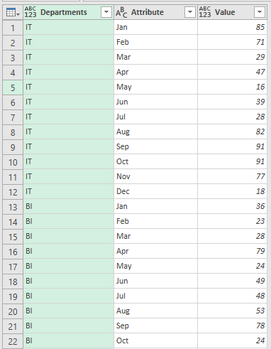
The next step is to rename the column Attribute to Month. be careful about any Change Type. You must delete them!
Whereas we could add additional steps doing calculations and further transformations of data, we will stop here and say that our query is now finished and therefore ready to be turned into function.
Creating the Custom Power Query Function
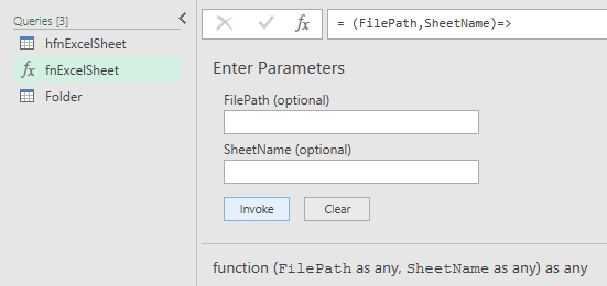
Duplicate the query with right click> Duplicate in the queries sidebar. Change the name of the new query to fnExcelSheet.
Now we open the Advanced editor. Add the following line to the beginning of the code:
(FilePath,SheetName)=>
Change all actual file paths and sheet names in the code to arguments FilePath and SheetName.
Confirm with Done. This Query just became a function.
We now need a list of file paths and sheet names to use the function. We create this list using the following steps.
Creating the Final Query
We make a new query with Right-click > New Query > File > Folder straight from the left Queries sidebar. Now select the folder where you have stored Excel files and chose Transform Data.

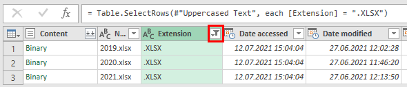
Since we can have other files stored in this folder we want to make sure only Excel files remain on this list. This is achieved by clicking on the Extension column filter icon and select ».xlsx«.
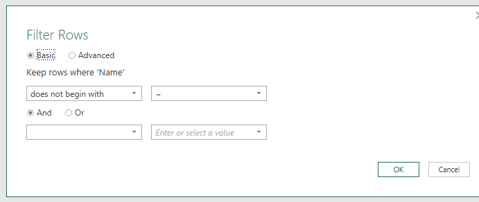
We also want to make sure not to use any temporary files Excel creates while using the original files. Once again we select the filter icon, this time on the Name column, and then Text Filters > Does Not Begin With..
We type in symbol ~ and confirm with OK.
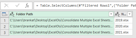
Now we are ready to remove all columns apart from Folder Path and Name by selecting the specified columns in the right order and right click > Remove Other Columns.
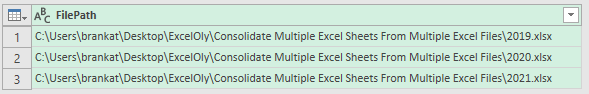
We then merge columns by selecting (again in the right order) both columns and Transform > Merge Columns.
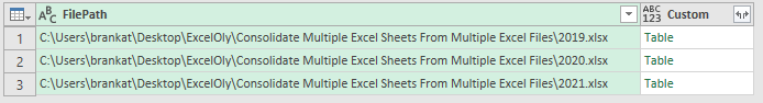
Now comes the magic part. We add calculated column with Add Column > Custom Column. Use the following formula: Excel.Workbook(File.Contents([FilePath]))
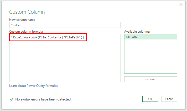
A column called Custom is created.
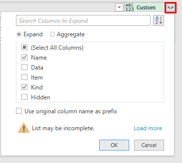
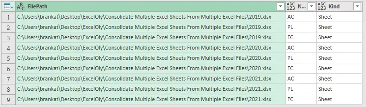
Click the Expand icon and expand the Name and Kind column.
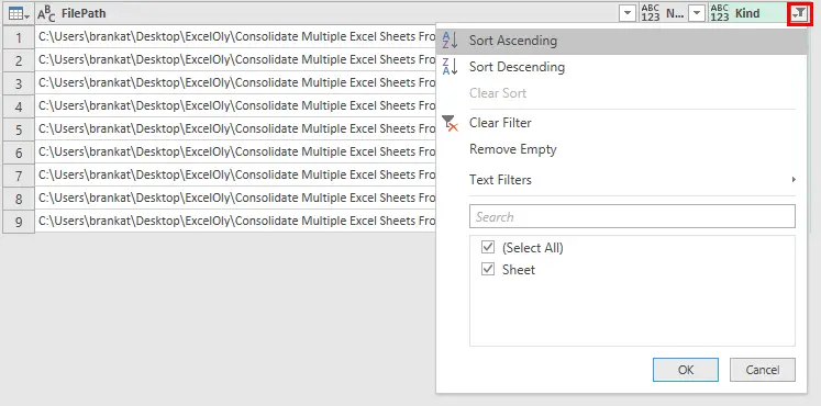
Since we have a function that works on Excel workSheets, we will filter the Kind column to Sheet.
Now we can remove column Kind.
Invoking the Custom Function
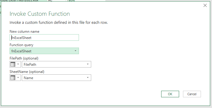
We are now ready to use our function. Select Add Column > Invoke Custom Function. Fill out fields as on the image below.
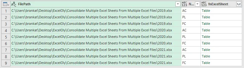
We get a column of all the tables.
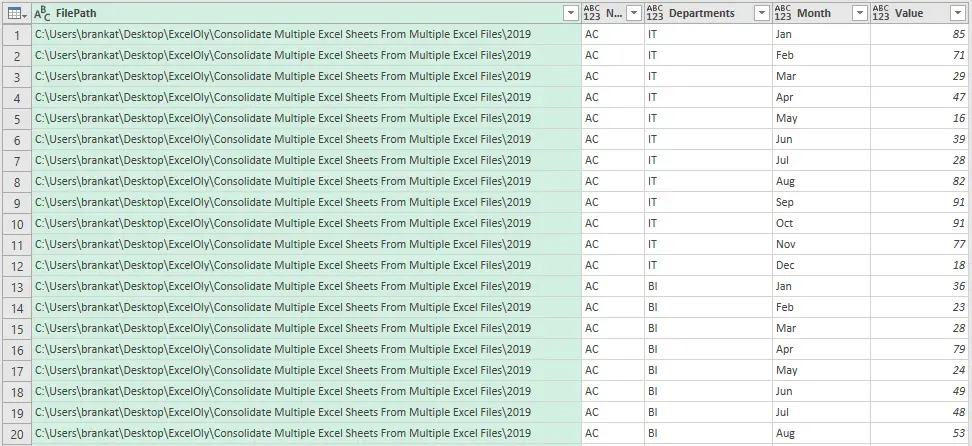
Select the Expand icon on fnExcelSheet column and expand the tables.
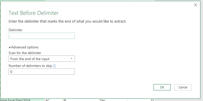
We don’t need the file path listed in the first column, we’d only like to keep the year. We extract the year by selecting Transform > Extract > Text Before Delimiter. We enter “.” as delimiter.
Similarly, we extract text after “/” delimiter with Transform > Extract > Text After Delimiter.
Lastly, we rename the columns.
And now we have a beautiful consolidated table derived from multiple Excel workbooks and multiple Excel sheets!
Watch the tutorial
Prefer watching? Learn how to consolidate data from all Excel sheets in multiple Excel workbooks by watching the following video:
Please leave us a like, comment, and subscribe for more amazing Excel tricks! Share with your friends to get all the Excel sheets in order.
Follow us on LinkedIn.
Check out our brand new R Academy!
Excel Unplugged acknowledgements


Donate
