Dynamic ranges in Excel
- Gašper Kamenšek
- October 9, 2013
- 4 Comments

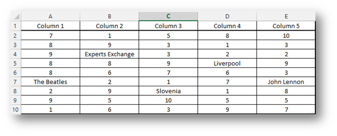
For the purposes of this article (if you wish to follow long and I strongly suggest you do so) we will be using a workbook that has the A2:E10 Range filled with the following random data.

In real life Ranges like this are very rare and very unkind to the user, since no column has unique format of data used (numbers and text are present in every column). Our goal is to set up a simple SUM function to add up the values in Column A, but to do this in such a way that every addition to the existing data in that column will be reflected instantly in our SUM. And just to clarify, not to insert new data between the old, but to insert new data below the last record.
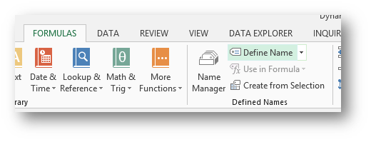
To create a so called dynamic range in Excel we must give that range a name. Usually we would do this by selecting the cells that make up the range and writing the name in the Name Box. Doing this in such a way would make our SUM function look better but it gives us no dynamics. So, to make the range dynamic we will add the name manually by using the Formulas/Define Name command.

This is the command we will be using. And let’s say that to start with we will only name the first column of data. So selecting A2 (since it’s where our range will begin) we fill in the following in the dialog box.
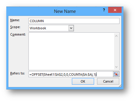
In the Name Field we put COLUMN (you can use anything you like but without spaces!). And in the Refers To we put
=OFFSET(Sheet1!$A$2,0,0,COUNTA($A:$A),1)

Let’s explain the function above.
The OFFSET function returns the reference to a Cell or a Range, that is for a certain number of rows and columns away from the current Cell or a Range. Where it can be used for a simple reference to a different range, it can also be used to create Ranges. Now for the purpose of distance from the cell we use the Rows and Columns arguments but for the purpose of creating a range, we give the Height and Width arguments.
Syntax: =OFFSET(range, rows, columns, height, width)
range the starting Cell or Range
rows the number of Rows to offset by. Can be both a positive or a negative integer.
columns the number of Columns to Offset By. As above, can be positive or negative.
height the number of Rows we wish the Range to contain
width number of columns the new Range should contain
Example:
=OFFSET(A1,1,2,1,1) gives C2
=OFFSET(A1,1,2,2,3) gives C2:E3
=OFFSET(C3,-1,-2,1,1) gives A2
This was more or less only the use of the Rows and Columns arguments of the OFFSET function. The Height and Width arguments were only used for the purpose of defining that we want the Range to be a single cell.
But in our example, the function was different. It went as follows.
=OFFSET(
no suprises so far Sheet1!$A$2
is the original Cell or Range, it can also be $A$2 or simply A2. Then we put ,0,0,
the commas are meant to separate the two arguments which are Rows and Columns and in this case both are 0, mean that the first cell remains in place, so no offset. The next part is a bit of magic on our part, it states COUNTA($A:$A). What this does, is it tells us how many rows is in the Range that the name COLUMN describes. Since we want this argument to actually count the rows used by the range, we could simply put the COUNT function there, but the problem would be, that the COUNT function only counts numbers where as our range contains both numbers and text. Therefor COUNTA is required for the counting of the cells that contain data. So it just counts how many cells have data, no mather of the data format. There is another trick we used in this function, that is to give the range as $A:$A. This helps us in not limiting ourselves right out of the starting blocks and will work for as many cells as it will take throughout column A.
After that we have ,1) . Nothing magical here, it just states that our Range is one Column in width. Followed be the parenthesis.
Now we can write our function
=SUM(COLUMN)
This adds up all the values in column A. If we were to add a new value below the last value, it would automatically expand our COLUMN range by that cell and automatically add that value to our SUM. Even if the value we were to add was a string, the range would have expanded since the COUNTA function counts cells that are not blank regardless of whether the cell content is value or a string. Needless to say the SUM would not change.
But there is a catch with using this. Let’s say our COLUMN range is now A2:A10. What if we were to leave a blank cell (A11) between the last value and the value we would be adding (A12). The range would still expand by one row (A2:A11), but since we left one blank cell in-between our previous data and the new value, that blank cell now becomes part of the range. What that means basically is that our new value is not included in the COLUMN range and therefor in our SUM. In this case the COUNTA function is not strong enough for what we want to do. Let’s redefine our named range using the following instead of COUNTA…
=MATCH(9,99999999999999E+307,$A:$A,1) when we wish for the range to automatically expand to the last cell with a value or
=MATCH(REPT(“z”,255),$A:$A,1) when we wish for it to expand to the final string value. This is paramount to the dynamic Data Validation lists.
In both cases the first values are exaggerated but they are the largest Value and the “largest” String that you can put into a cell and therefor will work in every situation.
Here’s how this works. The MATCH function will tell us where (row number or better yet a consecutive cell in a range) the last value that is still smaller than our 9,9E+307 lies. Now the range will automatically expand to that last cell and include it in the SUM or a Data Validation list.
And we are one step closer to eternal happiness.
Related Posts
- September 2, 2014
Our goal here, is to create a dropdown list by using Data ...


