Our goal here, is to create a dropdown list by using Data Validation, where the contents of the list will be determined by another Data Validation Dropdown list. Here’s an example…

Now there are two dropdowns here, one for the Band and another for the Song Title. But the Song Title dropdown should reflect our choice in the Band dropdown. So if I choose The Beatles as a Band, I want my Song Title dropdown to begin with Please Please Me and go through to Here Comes The Sun.

But if I was to choose Vintage Trouble as a Band, a different story should be seen…

Ok, now that we know where the train is heading, let’s get moving. If you want, you can follow with the original file

Dependent Data Validation dropdown lists.xlsx

We will achieve this in three steps.

First we will create a dropdown list in cell A3 to enable the band selection. Before attempting this, make sure, that the band names do not include spaces! It’s very important that the spaces were replaced with underscores. So instead of The Beatles, we have The_Beatles. It’s not that this is the only way, but there can be no spaces! I will explain later on, why that is. Now back to the first dropdown.

The first Data Validation dropdown list

Select cell A3 and Data/Data Validation

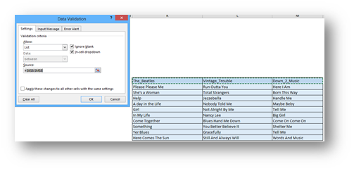
And you get the following textbox

Where you mark the cells with the Band Names as the Source. Press Ok and you should get…

Creating the named ranges

And now for the hard part or step 2. In our data table, all columns of data should get their names from the top row (the band names). We will let Excel do the hard work here. First, we select the entire table with the band names and song titles. Then we go to FORMULAS/Create from Selection and in the dialog box select Top Row, since the band names in the top row are the names we wish to give to the ranges.

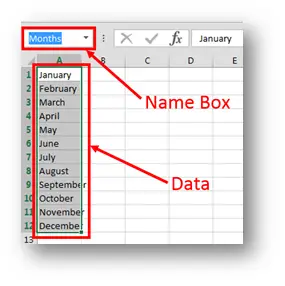
After you press OK, you should check the Name Box dropdown if all three names were applied. Do not be surprised by the sort order because it is alphabetical and can differentiate from the sort order in your table. The main thing is that the names were given and are the same as the ones in the top row of our table. With the underscores and all! If you didn’t follow the instructions for the band names, they must not contain spaces. If they did, spaces were automatically replaced with underscores by the Create from Selection command. If they are different now, correct the names in your table to match with the names of the ranges.

Creating the dependent Data Validation dropdown list

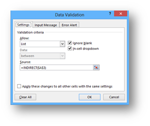
And now for our final step. Creating the second dropdown. Select the cell where you want the second dropdown to be (B3 in our example) and go to Data/Data Validation and then put =INDIRECT($A$3) as a Source

And that’s the whole magic. Since the A3 Cell contains the name of the range, the INDIRECT function understands that that range should be the source for the second dropdown. And when you change the selection in A3, the dropdown in B3 changes accordingly.

If you manage to combine this with the knowledge of Dynamic Named Ranges in Excel, then you really have something very powerful!

Extra step:

The one thing that can be unpleasant at this point is that if you already selected a song from the second dropdown, and you then change the band selection, although the second dropdown will change, the cell content will not. So the song you originally selected will remain there. It can be changed of course, but it is a nuisance brought about by the fact that Data Validation will check everything you put into that cell from this point on, but it will not check if what is already in a cell is compliant with the new validations. But this can be overcome by the use of VBA. If you are not comfortable with the use of VBA, don’t worry, this is not required for the dependent dropdown list to work, it’s just a cosmetic thing.

To make it work you will need two pieces of code. The first is very short and sweet. It’s a simple declaration of two variables that Excel needs to remember even when the code is not running.

 Global Bnd As String
Global acheck As Integer

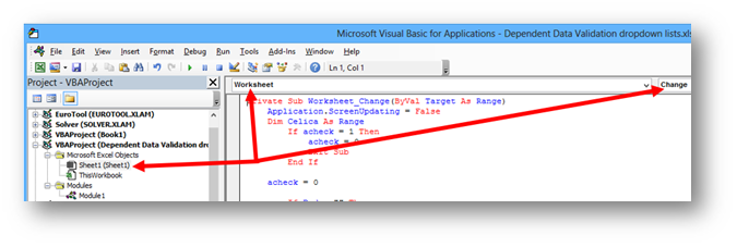
Now for the main code you need. This one you place into the WorkSheet code and attach it to the WorkSheet Change event.

Here’s the code (it relies on the example that is in all the screenshots. The placement of the dropdowns is important. If you have placed the two dropdowns differently, then you must change those ranges (A3 and B3) in the code). Do not copy this code (you can read why in the second comment bellow the post. Copy it out of this working sample of data validation with VBA.

 Private Sub Worksheet_Change(ByVal Target As Range)
Application.ScreenUpdating = False
Dim Celica As Range
If acheck = 1 Then
acheck = 0
Exit Sub
End If
acheck = 0
If Bnd = "" Then
Bnd = "The_Beatles"
End If
If Range("A3").Value <> Bnd Then
For Each Celica In Range(Range("A3").Value)
s = 0
If Celica.Value = Range("B3").Value Then
s = 1
Exit For
End If
Next Celica
If s = 0 Then
acheck = 1
Range("B3").Value = ""
Exit Sub
End If
Bnd = Range("A3").Value
End If
Application.ScreenUpdating = True
End Sub