Custom Cell Format You Must Know in Excel
- Gašper Kamenšek
- July 22, 2014
- 5 Comments
Custom cell formats are a very important steppingstone to eternal happiness in Excel. And among all Custom Formats, one takes precedence for both, its usability and versatility. We will get to understand it through two examples.
(If you like learning through video more that through reading, you can watch a Video I recorded for my YouTube channel that covers everything that you would learn in this blog post. Here is the link to the video : https://www.youtube.com/watch?v=YwmV-KNi6RQ. You can also view the same video embedded at the end of this post.)
Four for the Price of One
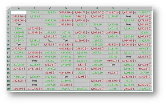
The following Custom format allows you to set four different formats at once. And the best part is, unknowingly, you’ve been using it since you’ve started using Excel. But now, you will understand it and be able to take it to the next level. Let’s start with a simple example. It’s a range of cells filled by positive and negative values, zeroes and text. It’s great if the positive and negative go above 1000 or bellow -1000, since this will better show the effects of our format. To create this I used =RANDBETWEEN(-10000,10000)*RAND() and if you preselected the range, give it a little Ctrl+Enter 🙂 Now the RANDBETWEEN function will only give you random numbers between -10000 and 10000. If you wish to have zeroes and text, you have to add them manually. Simply by selecting a few cells, writing zero and then Ctrl + Enter.

This is a very simple example of a range in excel that has positive values, negative values, zeroes and text. Now let’s try the following…
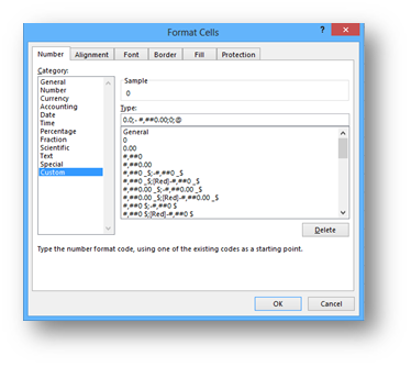
Select the range of cells and press Ctrl+1 to get the Format Cells dialog box (one of the best shortcuts in Excel, but the first time you use it can sometimes take a while). You can also right click and choose Format Cells…, or you can use any other method you would normally use.
Go to Custom and add type in 0.0;- #,##0.00;0;@
Press Ok and Voila…
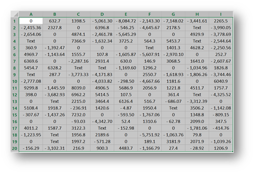
Here’s what we see:
- The positive numbers are all shown with a one decimal point precision and no 1000 separator. (0.0)
- The negative numbers are shown with a minus sign, two decimal points precision and a 1000 separator. (-#,##0,00)
- The zero values are shown with no decimal places and no 1000 separator. (0) This is something we wish to do on numerous occasions, to show zeroes differently that other numbers. Also, this is something that can be easily observed if you’re using the accounting format where the null values are shown as -.
- And finally, the text is shown. (@)
From this example we learned that it is possible to differentiate in Excel, how the positive, negative, zeroes and text will be formatted! The custom format looks like this.
Positive;negative;zeroes;text or sometimes it will be referred to as +;-;0;@
Here is a far more advanced example.
One more time we select the range and go to Format Cells… (Hopefully by pressing Ctrl+1) 🙂
This time the format will be
[Green] #,##0.00;[Red] #,##0.00 (-);;@
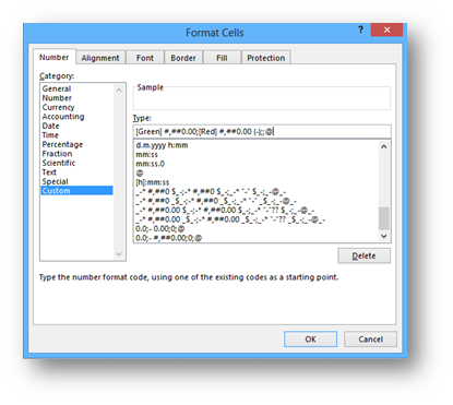
Here’s what we get

- So the positive numbers are green (if you chose a different language for your Office UI, then you must write the colors in that language), have a 1000 separator (if necessary) and two decimal places. ([Green] #,##0.00)
- The negative are Red, the number itself is formatted in the same manner as the positive numbers are, but with the addition of a minus sign in brackets at the end. Yes, you can do that to, if you wanted to, you could leave the minus sign out completely.
- Now here’s a shocker and one of the most useful things this format does. You can see that no format was set for the zero values and therefore, they are not visible. So if a format is not set, the values are hidden 🙂 Simply brilliant.
- Nothing special to say about the Text format, but if we omitted the @, no text would show. It would still be in the cell, but it would not show.
Now once you know this, you can do miracles and better yet, now you can understand the formats of the cells far better.
For example if you choose the simple Accounting format in Excel (which I guess you do every day), and then go to the Format Cells… and custom, you can see that what you really got is something like
_-* #,##0.00 $_-;-* #,##0.00 $_-;_-* “-“?? $_-;_-@_-
And there you have it. Four distinct formats and now we know why the zeroes show as -. There are some additional signs used to align the cells in the format above, but I will not get into that. My intention was to lay the groundwork here. If this topic interests you further, here is a great place to start.
Related Posts
- January 16, 2018
This is a follow up post on the final result of last week’s ...
- February 24, 2015
Surprisingly, this is not a post about the Translate feature in ...


