Simulating a “Tabular Form” Pivot Table Layout with Conditional Format
- Gašper Kamenšek
- January 16, 2018
- 0 Comments

This is a follow up post on the final result of last week’s post Table.Join function in Power Query. So basically, we want to get from this
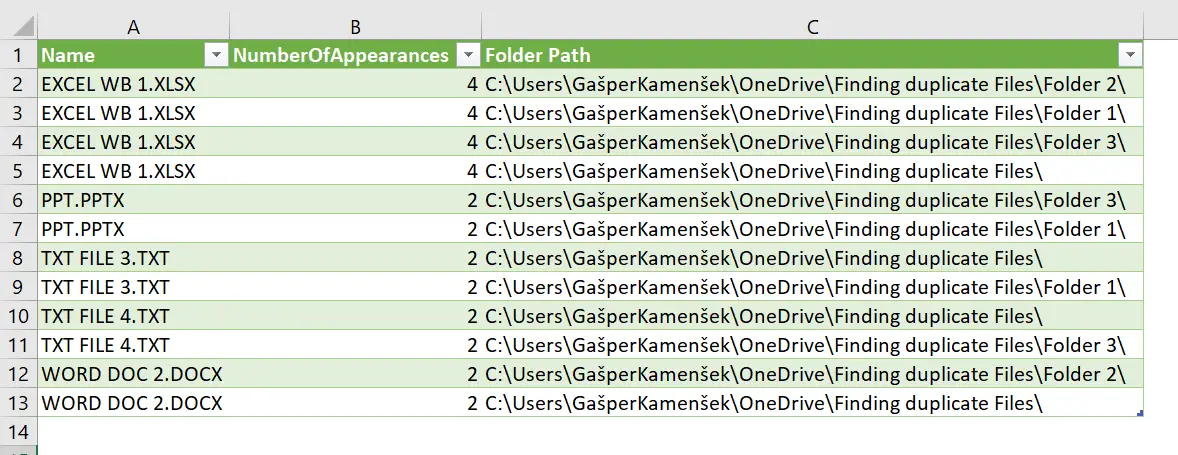
To this

Only by using Conditional Formatting.
First, we need to make sure, that the column in which we will be simulating blank cells (Name) is sorted correctly. We need to group the same filenames together…
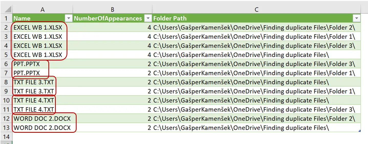
In our case, that was the result of Table.Join in Power Query and no sorting was needed, but in other scenarios, the table would have to be sorted by the Name column.
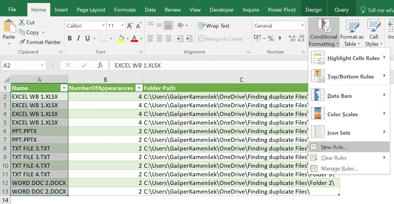
Now we can set up the Conditional Formatting rule, that will hide all filenames beyond the first for each unique filename. As with any Conditional Formatting rule, we start of by selecting the cells where conditional formatting will be applied. In our case that’s the first column (Name).
Then we go to Home/Conditional Formatting/New Rule
And in the New Formatting Rule we choose Use a formula to determine which cells to format
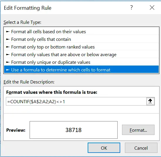
The formula we enter is
=COUNTIF($A$2:A2,A2)<>1
Which basically translates to Check if the current filename appeared more than once in a range from the beginning of the column and up to the current row. Now we set up formatting if the condition is met. We select the Format… button and on the Number tab select Custom and write the following custom Format code
0;-0;0;

The code says this: “Show positive numbers and show them rounded to a whole number, do the same with negative numbers and zeroes. But don’t (!!!) show text“. If you want to learn more about this custom cell Format, a great place to start is the following article:
https://excelunplugged.com/2014/07/22/custom-cell-format-you-must-know-in-excel/
And voila

Only the first appearance of each filename is shown and every successive one is hidden by the conditional formatting rule we’ve set up.
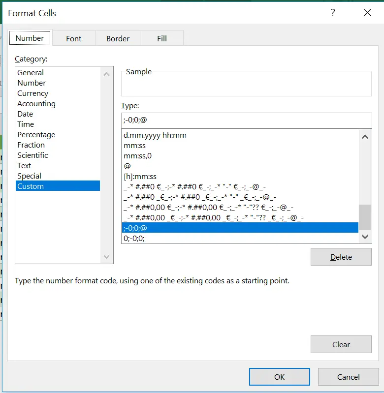
To achieve the same in the second column (NumberOfApperances), we repeat the process from above with two distinct differences. First difference being the selection of the column. We select the NumberOfApperances column and not the Name column. Then we follow the checklist from the first sample up to a point where we write the same formula…

And now we arrive at the second difference, the custom Format. This time the code will be
;-0;0;@
This one translates to: “hide positive numbers, show negative numbers rounded to a whole number, show zeroes and text“.
And once again, eternal happiness

Related Posts
- February 24, 2015
Surprisingly, this is not a post about the Translate feature in ...
- July 22, 2014
Custom cell formats are a very important steppingstone to eternal ...


