Convert Text to Numbers in Excel
- Gašper Kamenšek
- July 29, 2014
- 2 Comments
A task that comes about every so often in Excel and can be quite tricky. Now our ultimate goal is to get a number out of something like (text 1 text) or even (text123text). This is the main focus of this post but just to cover all the bases, let’s start with the easy stuff.
Value Function in Excel
=VALUE(text)
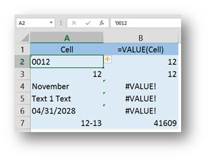
Built for exactly this purpose. It takes text and if it can, converts it to a number. For instance if a cell contains ‘0012 it regards that 12 as a text and gives you leading zeroes. Now if you put a VALUE on top of it you get 12 as a number. Here are a few examples…

Very straight forward, but it must be said that there are limits to what VALUE can do. For example it can convert a 12/01/2013 to 41.609 or ‘0012 to 12, but when it comes to a combination of text and numbers in a cell (Text 1 Text), it’s a NO GO (but do not despair, just keep reading).
Convert to Numbers Using Paste Special in Excel
As opposed to a VALUE function in Excel, this method does not require you to fill any extra cells, and allows you to convert text to numbers on the fly. Here it is…
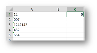
Column A has many numbers that were imported as text. To convert them to numbers, we begin with a 0 (zero) value in a cell. Then you act as if you want to copy that cell, so Ctrl+C, right click and Copy… Now here comes the tricky part. You select all the cells you wish to change to values…
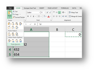
…and choose Paste Special…

And select Add in the Operation group. This will add the value of a cell you were copying (zero) to all selected cells. And then something great happens. Since Excel has to calculate with those cells, it realizes that the content of those cells must be a value. And it immediately converts all those cells content to numbers. As simple as that.

You could achieve the same by choosing Subtract or by copying 1 and choosing Multiply or Divide.
But still, if a combination of text and number (text 1 text) is in a cell, it still won’t turn it into a number. Now here comes the hard stuff
Extracting numbers from a text-number combinations in a cell
We will do this in two ways, with a “simple” formula and later with VBA.
The formula is
{=VALUE(MID(A5,MATCH(1,(–(ISNUMBER(VALUE(MID(A5,ROW(INDIRECT(“1:”&LEN(A5))),1))))),0),SUM((–(ISNUMBER(VALUE(MID(A5,ROW(INDIRECT(“1:”&LEN(A5))),1))))))))}
🙂

We will go one step at the time, but first of all, notice the curly brackets at the beginning and at the end. That means that this is an Array formula, it has(!!) to be entered by a Ctrl+Shift+Enter combination and it has to be entered without the curly brackets(!!!).
The core of the entire function is the following
(–(ISNUMBER(VALUE(MID(A5,ROW(INDIRECT(“1:”&LEN(A5))),1)))))
And this is repeated twice throughout the formula
{=VALUE(MID(A5,MATCH(1,(–(ISNUMBER(VALUE(MID(A5,ROW(INDIRECT(“1:”&LEN(A5))),1))))),0),SUM((–(ISNUMBER(VALUE(MID(A5,ROW(INDIRECT(“1:”&LEN(A5))),1))))))))}
Here’s how it works…
The base of it is the MID function. The Mid function starts with the string in A5 and braks it apart to individual characters. It does that with the second parameter, which is basically a ROW(1:14) but it’s written dynamically. So the 14 is given by the LEN(A5) function and would change if the length of a string in A5 changes. Indirect puts the “1:” and 14 together for the ROW function. So MID {=MID(“Text 18764Text”,ROW(1:14),1)} gives you this {T,e,x,t, ,1,8,7,6,4,T,e,x,t}. So it breaks the string apart.
Now over this, you send the VALUE function. This is just to ensure, that the numbers will be numbers and not text. An important step before the ISNUMBER function takes over. The ISNUMBER function will return a (False,False,False,False,False,True,True,True,True,True,False,False,False,False). The (–( in front of it will change that False and True statements into zeroes and ones (0,0,0,0,0,1,1,1,1,1,0,0,0,0).
So, now we understand the core, let’s see what was put around it. In the first case, it was MATCH, to find the first appearance of 1 or in other words, the position where the number begins. In the second case, it’s SUM. SUM allows us to count how many numbers there are. What it also does, it destroys the formula, if more than one numeric values are present.
So now we know that the outside MID looks like this
=MID(text, where the number begins, how many numerals there are)
Since MID is a text function in Excel, the result of MID is once again wrapped in VALUE, so that the final result is a number.
It’s worth mentioning, this only works, when only one(!!!) number is hidden in the string.
VBA code to extract a number from a string
This will be a User Defined Function or UDF called GetInteger. As the name suggests, Integer is all you can get. No decimal places! One could have some fun with it further on, to add the decimal functionality, but the logic and the basic code is all here.
 Function GetInteger(s) As Double
Length = Len(s)
st = ""
For i = 1 To Length
zn = Mid(s, i, 1)
If (IsNumeric(zn) Or (zn = "-")) Then
st = st & zn
Else
If (st <> "") Then
If Right(st, 1) = "-" Then
st = Left(st, Len(st) - 1)
GetInteger = CDbl(st) * -1
Else
GetInteger = CDbl(st)
End If
Exit Function
End If
End If
Next i
GetInteger = CDbl(st)
End Function
Hope this gets you one step closer to eternal happiness in Excel 🙂
Related Posts
- January 26, 2016
The title of this post is actually a question I got on one of the ...
- November 11, 2014
As promised in the Pragmatism vs. Purity in Excel article from ...
- June 24, 2014
This will be a short lesson on three great and sadly unknown ...


