Sum up the diagonal of your data anywhere on a Sheet
- Gašper Kamenšek
- January 26, 2016
- 2 Comments

The title of this post is actually a question I got on one of the last trainings I gave in 2015. It struck me as a great little sample of using array formulas, and simply a demonstration of how array formulas can be a great time saver.
So let’s start with a sample data and let’s start simple so that data starts in cell A1.
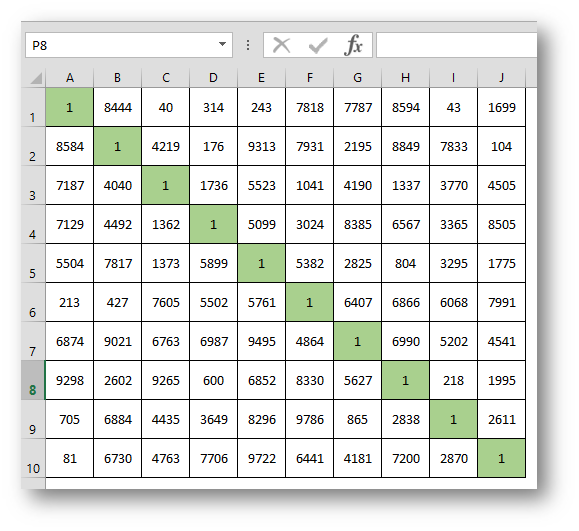
Also to make things easier I used a 10×10 matrix and filled all cells on the diagonal with ones. So the sum should be 10. Here’s the starting formula
=SUM(A1:J10*(ROW(A1:J10)=COLUMN(A1:J10)))
Now the most important thing with this formula is that you enter it with a Ctrl+Shift+Enter key combination since it is an array formula.
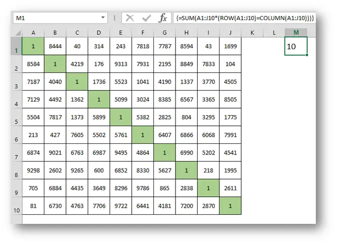
As we can see, we get the expected results.
Let’s dig into the formula. The key to its simplicity lies in two functions that we used, the ROW and COLUMN. Both of these just take a cell and return a number of the row or column in which the cell resides. So in the center of the formula, we have a ROW(range)=COLUMN(range). The reason we’re using this condition is the observation that the diagonal cells are the only ones where the row number is equal to the column number. This condition gives us a bunch of TRUE and FALSE values or you might look at theme as 1s and 0s. So when you multiply this with the values in the cells, only the diagonal values remain, all the rest return 0. Then as we throw the SUM function over that, what you are left with is the SUM of all diagonal values.
Ok, so that was the easiest sample but now let’s look at hoe the formula changes if the range is offset by n rows and m columns.
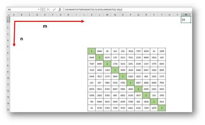
Now all we have to do to make our formula work is to somehow change the formula so that the n+1 row becomes 1 and m+1 column becomes A or 1. So to sort of move the range back to start in A1. We can do this two ways. The easier and the one that requires no thinking is that we simply retract n from all the rows and m from all the columns. So the new formula would look like this
=SUM(K6:T15*((ROW(K6:T15)-n)=(COLUMN(K6:T15)-m)))
This also gives us the general formula for this
=SUM(range*((ROW(range)-n)=(COLUMN(range)-m)))
Now the second way is to retract the difference between n and m from the largest of them. In our sample that is m and the formula would be
=SUM(K6:T15*(ROW(K6:T15)=(COLUMN(K6:T15)-(10-5))))
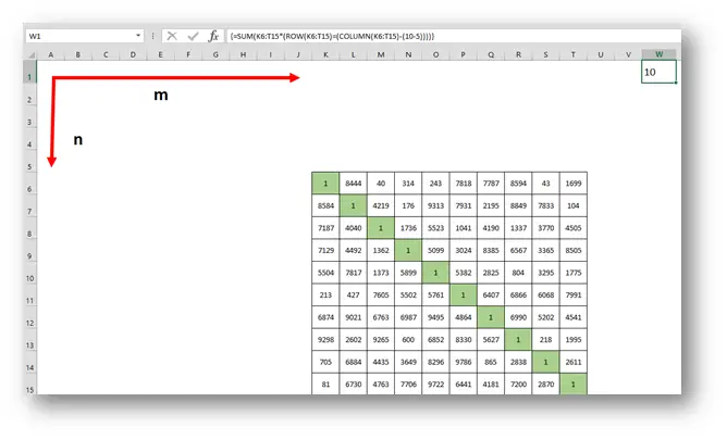
As we enter either of the two formulas with the Ctrl + Shift + Enter combination we get the result you see above.
And yet again we are one step closer to eternal happiness.
Related Posts
- November 11, 2014
As promised in the Pragmatism vs. Purity in Excel article from ...
- July 29, 2014
A task that comes about every so often in Excel and can be quite ...
- June 24, 2014
This will be a short lesson on three great and sadly unknown ...


