On many occasions we would like to somehow get the dates belonging to the last day of current, previous or any other month, the first day of this month or any day of the current month. This post will show you a nice trick how to do that. Whereas for the last dates of the given month the go to function in Excel would have to be EOMONTH (End Of Month), we will show a neat trick how to do this with a well-known Excel function called DATE.
First off, let’s say we would like to get the date belonging to the last day of the previous and the last day of the current month.
Now with EOMONTH that would go
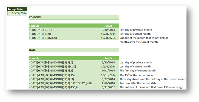
Last day of the previous month =EOMONTH(TODAY(),-1)
Last day of the current month =EOMONTH(TODAY(),0)
You can fiddle with the last argument to get to any month between Jan 1900 and Dec 9999. Keep in mind, that the EOMONTH function gives you only the serial number of the date, which you then have to format as a date.
It should be said that the DATE function gives you more leeway than EOMONTH since it can return literally any day of the month you choose.
=DATE(year,month,day) gives you the date you need or better yet the serial number belonging to the date you need.
For Example =DATE(2014,10,28) gives you 12/28/2014
But here’s a kicker =DATE(2014,10,0) gives you 9/30/2014
So with DATE function, these would be the two formulas (considering our initial goal)
Last day of the previous month =DATE(YEAR(TODAY()),MONTH(TODAY()),0)
Last day of the current month =DATE(YEAR(TODAY()),MONTH(TODAY())+1,0)
Now this trick with the zero as the last argument of the date function is genius. But even better, it can even go into negative. So you can do =DATE(YEAR(TODAY()),MONTH(TODAY()),DAY(TODAY())-2) gives you the date of two days ago.
Here are a few more examples of how you can use both functions
I can already hear you screaming what about the +1 on the month argument of the DATE function if the current month is December. Well you needless worry about that, you can easily go over 12 and the DATE function simply returns the month using the remainder after the number has been divided by 12 and even adds the number of years it get’s from the division by 12 to the year argument. Simply Brilliant and a great way towards that ever elusive Eternal Happiness.
Check out our YouTube channel and subscribe for more amazing Excel tricks!
Follow us on LinkedIn.
Check out our brand new R Academy!
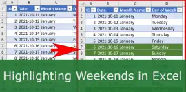
Highlighting Weekends can be hard in Excel. So just for fun, ...
This site uses Akismet to reduce spam. Learn how your comment data is processed.
=Today()-2 is a slightly easier/quicker way to get the date 2 days ago.
How would you calculate the first day of any prior month given TODAY()?
To make it interesting and bulletproof I would go with
=DATE(YEAR(EDATE(TODAY(),-1)),MONTH(EDATE(TODAY(),-1)),1)
Now only change the -1 to get to months further back…
Hope this brings you one step closer to eternal happiness 🙂
can you tell me how to get the next working day after the 20th for the previous month when the current date is shown in cell A1
=IF(WEEKDAY(DATE(YEAR(A1),MONTH(DATE(YEAR(A1),MONTH(A1),0)),21),2)=7,DATE(YEAR(A1),MONTH(DATE(YEAR(A1),MONTH(A1),0)),22),IF(WEEKDAY(DATE(YEAR(A1),MONTH(DATE(YEAR(A1),MONTH(A1),0)),21),2)=6,DATE(YEAR(A1),MONTH(DATE(YEAR(A1),MONTH(A1),0)),23),DATE(YEAR(A1),MONTH(DATE(YEAR(A1),MONTH(A1),0)),21)))
This juat might be the longest formula that will get you there but it is bulletproof…
Thank you very much.
is it possible to add on to an existing formula -1 work day ?
You could use the Workday function like =Workday(formula above,-1) and you could even add holidays as the third optional argument…
thanks
I should have said the 1st working day after 19th in my original request but I’m not sure how to adjust the formula?!
if A1=15/12/16 and I add -1 to the formula it provides the answer as Sunday 20 November but I would expect Friday 18 November or Monday 21st November
is it possible to get the expected answer?
The 18’th has me somewhat confused since it’s not after the 19th? If you really want the first workday after the 19th use the formula from before but change all 21 to 20, 22 to 21 and 23 to 22…
I am just trying to make simple calendar and I have put two input for the same I.e year and month how to get all the dates in columns for the same. Like I have 31 columns and in Feb only 28 days is there so other three column should remain blank. Thanks in advance.
Something like this
=IF(ROW()>DAY(DATE(2017,1+1,0)),””,DATE(2017,1,ROW()))
And just copy down…
this is for January 2017… And the formula should start in A1 and go down the A column. If you start lower (like in A5) you should do ROW()-4 (so that you get 1 in row 5. Otherwise the plus 1 in the first date function is important as the whole DATE function gives you the last day of the given month (read more about that at https://excelunplugged.com/2014/10/28/last-day-of-previous-month-excel/ )
and if you get to the nonexistent dates, the IF function kicks in and gives you a blank cell…
If the date is after the 20th of the month, I need to calculate the 20th of the next month. If it is before or on the 20th of the month, I need to have it returned the 20th of the month. For example if the date is 1/25/2019 I need the date return of 2/20/19. If the date is 1/15/2019 I need the date return to be 1/20/2019.
What would the formula be?
IF you have the date in A1, then the formula should be something like
=IF(DAY(A1)>20,DATE(YEAR(A1),MONTH(A1)+1,20),DATE(YEAR(A1),MONTH(A1),20))
And be really impressed with the way Excel handles the obvious outlier, December 🙂
Hi Gašper,
Is it possible to add text to the Last day of the previous month function in Excel without it changing to the serial number of the date? I’m trying to create a formula similar to, =”Customer spend from 03/20/21 – ” & EOMONTH(TODAY(),-1) , but the formatting is changing the last day of last month to a serial number.
You need to wrap your EOMONTH into TEXT so it would be TEXT(EOMONTH(TODAY(),-1),”mm/dd/yyyy”)