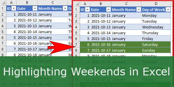
Highlighting Weekends can be hard in Excel. So just for fun, we’ll do this in three different ways: we’ll use conditional formatting to highlight the weekend dates in a column. Secondly, we’ll then use conditional formatting to highlight the entire row in a table. In conclusion of this post, we’ll level up and use the Lambda function to highlight the whole row in a table. Let’s do this!

Highlighting Weekend Dates Using Conditional Formatting

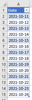
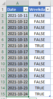
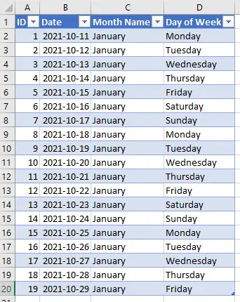
First, let’s start with a column of dates.

We add a column WEEKDAY and enter the following formula.

= WEEKDAY([@Date])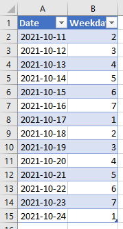

The week starts with Sunday in the US, so one represents Sunday, and 7 represents Saturday. We wrap the formula in the OR() function and state we are only interested in weekdays values 7 or 1.

= OR(WEEKDAY([@Date])=7,WEEKDAY([@Date])=1)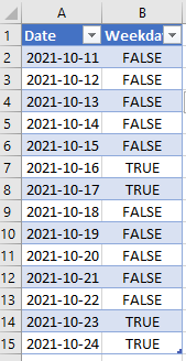

As a result, we have now found the dates occurring on weekends. Therefore, we can now use this function to create conditional formatting.

Firstly, we select the Date column (this is a crucial step and should not get overlooked as Conditional Formatting will only apply to the area you have selected!).

Select Conditional Formatting > Highlighting Cells Rules > More Rules.

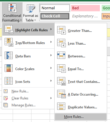
After that, we select Use a formula to determine which cells to format.

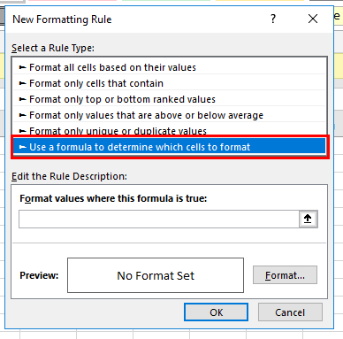
Enter the formula.

= OR(WEEKDAY(A2)=7,WEEKDAY(A2)=1)

Click the Format button in the preview below and set Fill color to green and Font color to white.

To sum up, confirm all with OK.

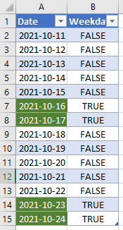
We can now remove the Weekday column and enjoy our neatly formatted Date column!

Highlighting Entire Rows with Weekend Dates Using Conditional Formatting

Similarly, we now have a table of dates with some additional attributes. We want to highlight entire rows in our table. The process is very similar.

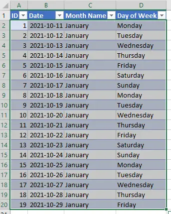
Firstly, select the table.

Secondly, select Conditional Formatting > Highlighting Cells Rules > More Rules.

Select Use a formula to determine which cells to format.

Enter the formula.

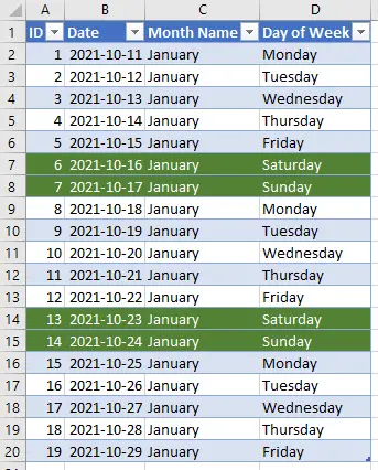
= OR(WEEKDAY($B2)=7,WEEKDAY($B2)=1)

The formula is the same as before, and we only added an absolute reference to the B column using the $ symbol. This means Excel will always check the B column and the corresponding row for each cell in our table and format accordingly.

Again click the Format button in the preview below and set Fill color to green and Font color to white.

Confirm all with OK.

Highlight Weekend Dates Using Lambda Function

We’ll now level-up and create a new function to use in our conditional formatting.

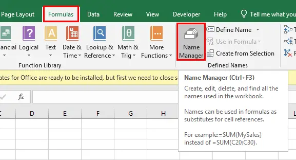
Select Formulas > Name Manager > New.

We obviously it BestThingEver and enter the formula, wrapped in LAMBDA() function.

= LAMBDA(a, OR(WEEKDAY(a)=7,WEEKDAY(a)=1))

We’ll use letter a as an input parameter.

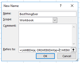
Confirm with OK.

The process from here on is similar to before. We select the table.

Select Conditional Formatting > Highlighting Cells Rules > More Rules.

Select Use a formula to determine which cells to format.

Enter the formula.

= BestThingEver($B2)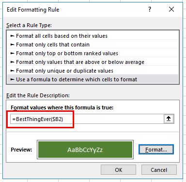

We again have our formatted table.

Easy as an apple pie!

Watch the Video Tutorial

We know some of you prefer to watch the mastery live, and we have this one for you in the video as well. You can find the video version of this tutorial here: https://www.youtube.com/watch?v=GFVOI6yHwz8

Please leave us a like, comment, and subscribe for more amazing Excel tricks!

Follow us on LinkedIn.

Check out our brand new R Academy!

Read related posts:

• Todays Date and Current Time Shortcuts in Excel

• Create a Date Series of all weekdays in Excel (omits Saturdays and Sundays)

• Formula to get the Start or End Date of the week