Filtering a Table to a List of Values in Power Query or Power BI
- Gašper Kamenšek
- March 31, 2020
- 42 Comments
Utilizing Power Query Lists Series – Part 1/3
Lists are (in my humble opinion) the most underrated output of Power Query. So rarely do we use them on purpose, and yet, we use them all the time since Power Query writes a new line of M code every time you click any command in the graphical user interface (GUI). Very often, those lines of code will contain Lists (most Common steps to do so are Changed Type steps). You should always keep a lookout for the curly braces as those indicate a list of values being passed to an M function. This post will focus on Filtering a Table to a List of Values, but in the entire three posts series, we will look at how we can use lists to do the following:
- Dynamically Filtering a Table to a List of Values (This post)
- Changing a Table of Attributes and Values to retain only Top 10 Attributes (by values) and turns the rest to Others
- Dynamically retaining only columns that contain Actual amounts from a Table
You can get the Workbook here and follow along.
If you prefer learning through video, you can watch this video or view the video embedded at the end of this article.
The Workbook
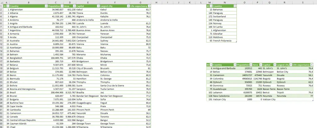
We start with two Tables. Table AllCountries contains a list of Countries plus some demographic data and looks like this.
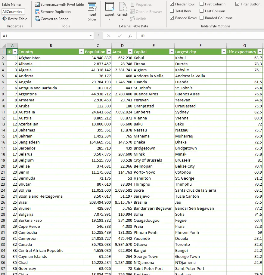
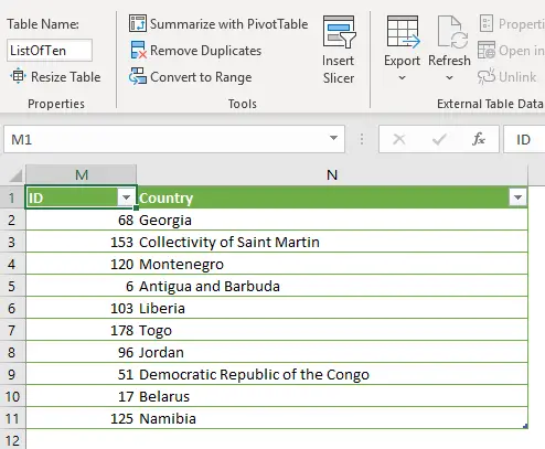
Table ListOfTen is just a random list of 10 countries from the main Table and looks something like this (the Id’s are calculated using RANDBETWEEN (in Office 365 with Dynamic Arrays there are far better ways to do this, but I used RANDBETWEEN so that all the steps apply to Excel 2010 and above)).
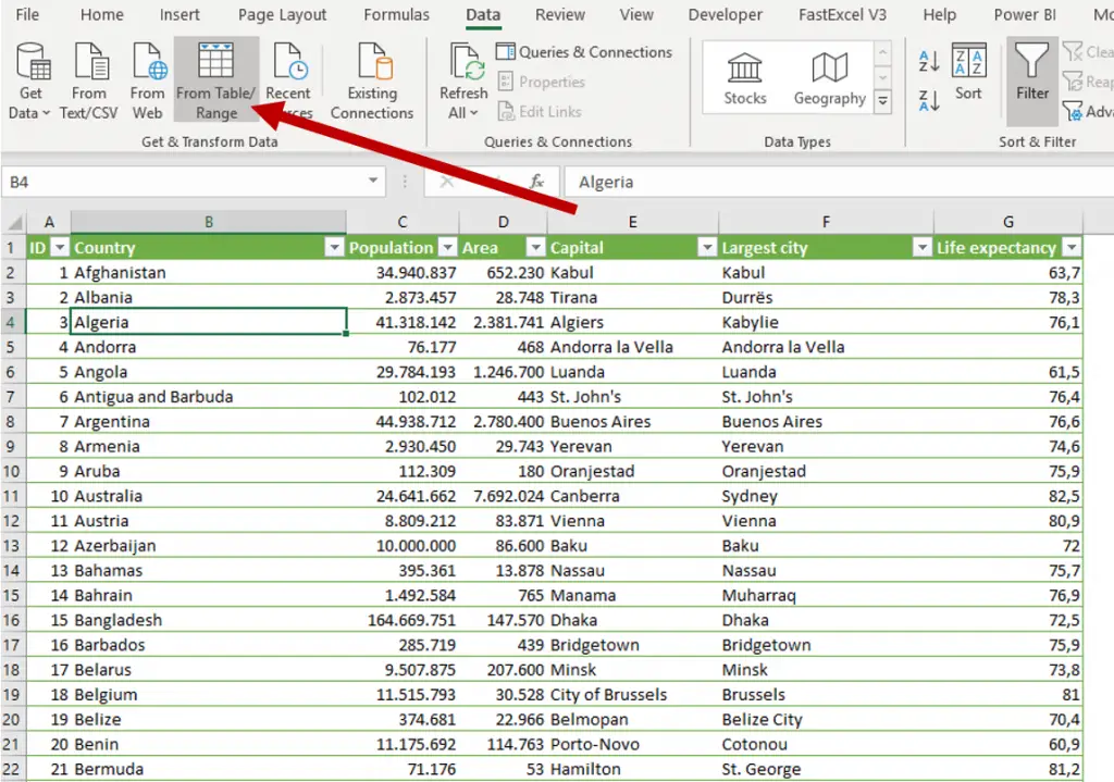
We get both tables into Power Query by selecting a single cell within the tables and clicking on Data>From Table/Range.
Consequently, we should end up with something like this.
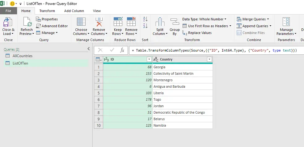
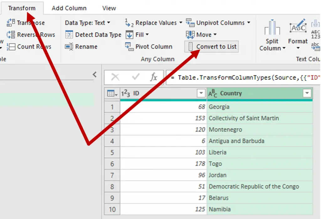
Now comes the important part. We must convert the list of ten countries into a list. We do this by selecting the Country column of the Table ListOfTen within the Power Query Editor and selecting the Transform>Convert to List command.
You should now see a noticeable change in the icon of the ListOfTen Query, suggesting that it is no longer returning a table but a list of items.
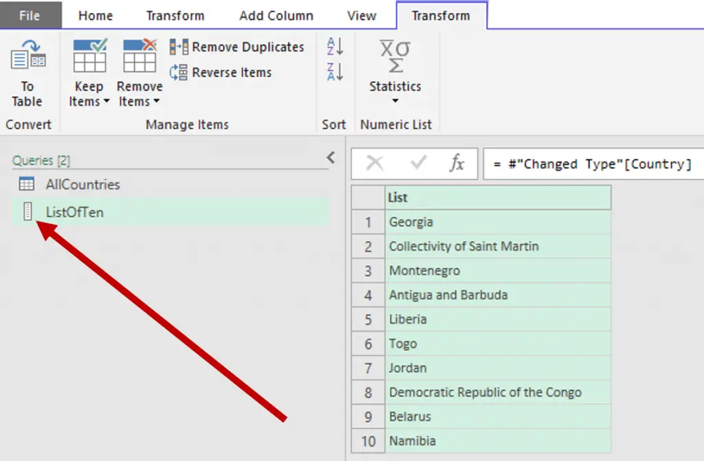
This means we now have a dynamic list of ten countries. The next step is to Filter a Table to a list that we just created.
Now we shift to the AllCountries Query and only select a few countries. The idea here is that we wish to get most of the code that we need for the next step.
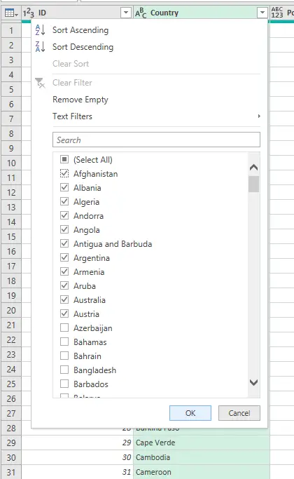
You should now see something like this in the Formula Bar.

We will only need this part of the code
= Table.SelectRows(#"Replaced Errors", eachAnd delete the rest.
Now we will replace the deleted part with
(List.Contains(ListOfTen,[Country])=true ))And we should see something like this

Here is the code of the entire step:
= Table.SelectRows(#"Replaced Errors", each (List.Contains(ListOfTen,[Country])=true ))And voila, we now only see the countries from our list.

After loading, this is what you get.
To clarify, if we replaced the true with false, we would exclude all the countries in our list from the result, which is just brilliant.
In conclusion, this was sums up Part 1 of the series. Stay tuned for the following parts!
Watch the tutorial
Here is a YouTube video explaining all the steps in detail.


