Extract Columns that Contain Actual Values
- Gašper Kamenšek
- April 28, 2020
- 2 Comments

We often work with large datasets containing multiple columns, but only need a few. In this tutorial we’ll show how to extract the columns that contain Actual values from your dataset. We’ll be using Power Query.
Utilizing Power Query Lists 3/3
This article is part 3 of the Using Power Query lists series. In this series, we will look at how we can use lists to do the following:
- Dynamic Filtering on a Column Using Lists
- Changing a Table of Attributes and Values to retain only Top 10 Attributes (by values) and turns the rest to Others
- Dynamically retaining only columns that contain Actual values from a Table (This post)
Similarly as with first two parts, we will be using the Dynamic Lists Retaining Columns Workbook for this article. You can get the Workbook here and follow along.
The Workbook
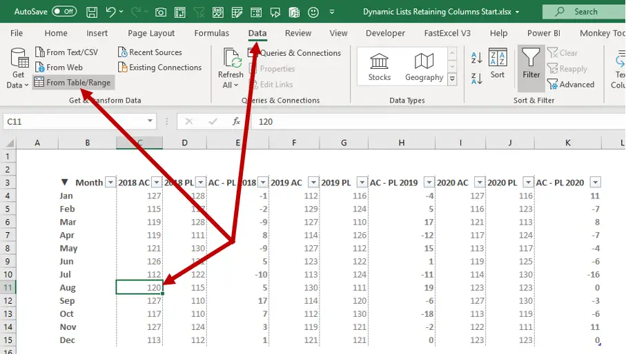
This time around, the Workbook is as simple as it gets as it only has one Table called ACvsPL. We have monthly data for three years and contains Actual, Plan, and the difference between the two. The Table looks like this.

We want to use Power Query to only return columns that contain Yearly Actual data and to do so dynamically. Most importantly, the key here is Dynamically(!), which means that if we let the query run on multiple Workbooks or WorkSheets with multiple tables containing a different number of Actual columns, this method will still work.
As a result, we are trying to get this.

And just to keep things interesting, our Table also contains the “AC – PL YEAR” columns. So we have two types of columns containing AC, and this will make our filtering a bit more complicated.
Get data from Table/Range
We start by adding the ACvsPL Table to Power Query by selecting any cell within the Table and using the Data > From Table / Range command.

Special apology to Ken Puls for cutting his Monkey Tools add-in out of the ScreenShot 😊.
The Query
First of all, when you get into the Power Query Editor, there is a chance that you are looking at two query steps or just a single one. The two steps include Source and Changed Type step. Power Query added the Changed Type step automatically. Therefore, we will include an extra step, just so that we will all be on the same page. We do so by simply clicking the fx icon in the formula bar.

As a result, this creates a custom step that is referring to the last step. Hence, we now all have either two or three steps, and the last step is called Custom1.
Getting the List of Columns with Actual values
Next few steps will be all about getting the List of columns containing the Actual values. First of all, we should have the header row containing the column names as a Column. Maybe you know the Command we are looking for from Excel. It’s called Transpose. But before we can transpose our Table, we need to demote the header row because the Transpose command turns rows into columns ignoring the header row!
Therefore we will use the Tranform>Use First Row as Headers (dropdown)>Use Headers as First Row.

Maybe you’ve never heard of this Command, but it has its uses, and it works beautifully with Transpose. You should now be looking at this.

Now we use the Transpose command. You will find it on the Transform tab, Transform > Transpose. This is what we get.

While the result looks much closer to what we need, it still needs some cleaning up. As we only need the first column, we right-click the header Column1 and select the Remove Other Columns Command.

If it wasn’t for the “AC-PL YEAR” columns, all that would remain for us to do would be a simple filter with the “AC” keyword. But since we made life complicated for ourselves, we will need to somehow differentiate between “YEAR AC” and “AC–PL YEAR” columns. We could make even more interesting by having “AC YEAR” columns where we would need to add a column with text length to differentiate between them, but as it stands, the columns we need are the ones that end with “AC”. So we go to Filter>Text Filters> Ends With…

And type AC as the value.

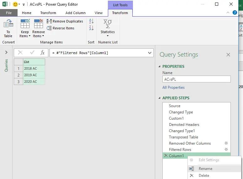
Finally, here it is. A list of columns that we want. But wait a minute… It’s not a list is it? Let’s make a list out of it. By going to Transform>Convert to List.

And there we have it. Our List in all it’s glory. Now let’s rename the last step Column1 to MyList.

Putting in all together
Now that we have our List saved as MyList and waiting to be used, let’s go back to our original Table. We simply click on the fx icon in the Formula Bar and type =Custom1.

As a result, we get our original Table (the result of Custom1 step) back.
Now we select the first three columns, right-click in the header and click on Remove Other Columns.

Most noteworthy, it doesn’t matter which (or how many) Columns we selected. All we are after is the code that this step will produce. And it should be similar to this.
= Table.SelectColumns(Custom2,{"Month", "2018 AC", "2018 PL"})Now, do you notice how the Column names are in curly brackets? This should be the most beautiful thing in the world right now as it means that this is a List of Columns. Now all we need to do, is to replace this List with our List. Remember, we saved it as MyList. So delete the curly braces and everything they contain and replace them with MyList. You should get this.
= Table.SelectColumns(Custom2,MyList)
And above all, you should get this.

Now we made this step dynamic. If there were ten “YEAR AC” columns, we would now be looking at ten columns.
In Conclusion
Although this was a straightforward example, you can use the steps described in this post:
- Create a step to reference the Table later
- Demote the header row
- Transpose the Table
- Keep only the first Column as that is a list of Columns from the original Table
- Use Filters, Sorting, Indexing, Custom Columns… to get to the List of desired Columns
- Change this List of Column into a Power Query List and rename the Step
- Use the List as a parameter of the Table.SelectColumns M function.
I use this method every time I need to reference a Sheet in Excel and get an endless number of empty Columns, which Power Query somehow thinks are in use. This method works perfectly, and since it’s dynamic, it goes hand in hand with Power Query functions and later on with the Unpivot Columns command.
And just like that, we are one step closer to eternal happiness 😊.
You can download the Workbook with the end result here.
Learn more
Check out our YouTube channel and subscribe for more amazing Excel tricks!
Follow us on LinkedIn.
Check out our brand new R Academy!
Related Posts
- April 14, 2020
How to get the top 10 values in a table, and an aggregate for all ...
- March 31, 2020
Knowing how to use Lists in Power Query or Power BI is like a ...


