R Language Overview and R Language Examples
R Language Introduction and R Language Examples
R is a programming language and software environment for statistical computing and graphics. It is free and open-source. It first appeared in 1993 and has gone through a number of releases. Today R is widely used for data analysis among statisticians and data scientists.
Further, R is a language designed specifically for data analysis and plotting. This differentiates R from Python in the sense that you may find algorithms and functions in R that are not yet covered in Python.
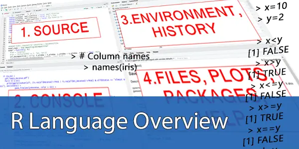
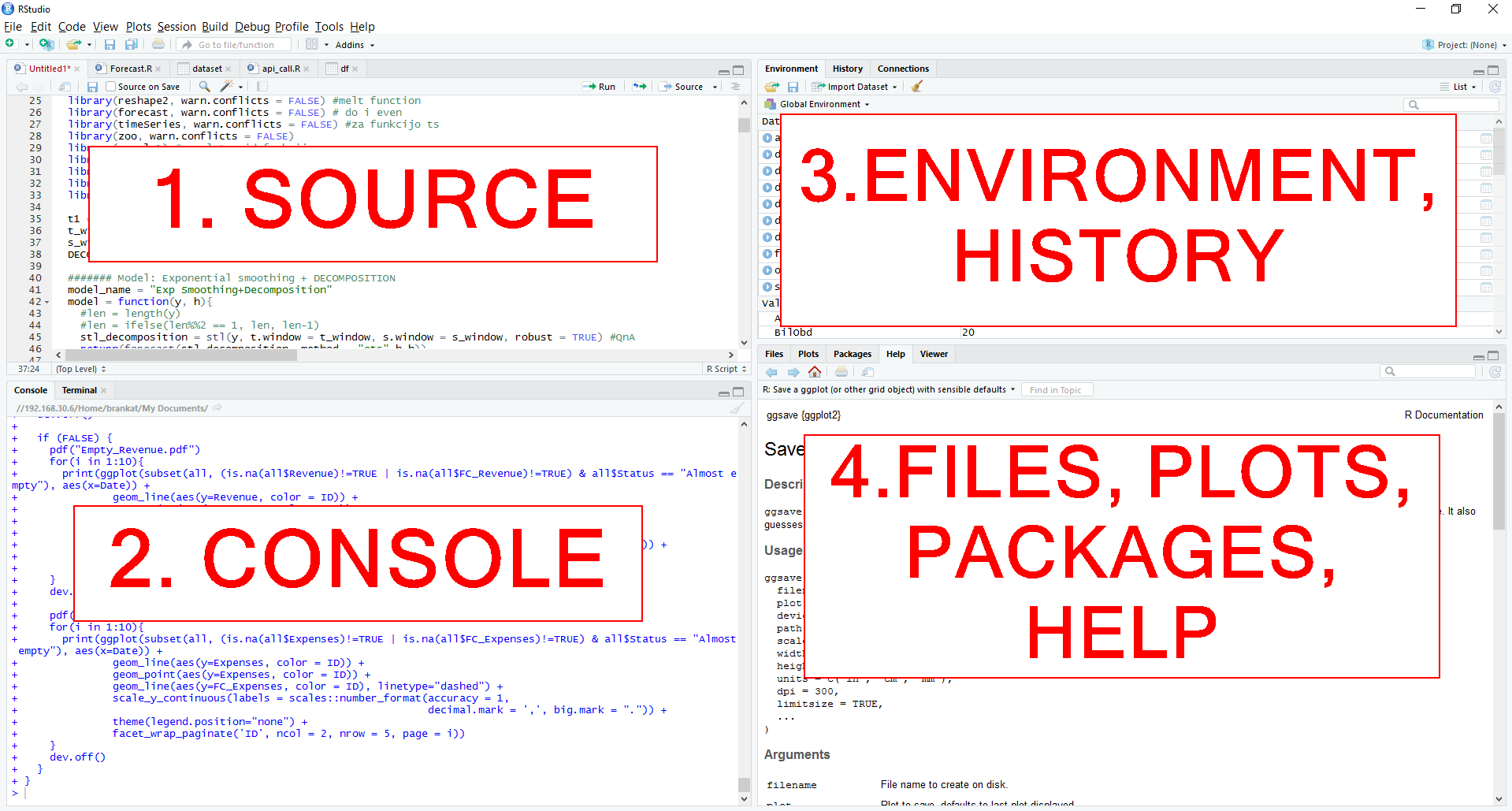
RStudio
RStudio is a free environment for R scripting. You can download RStudio at https://www.rstudio.com/.
RStudio workspace consists of 4 panes:
- Source Pane for viewing and writing R scripts
- Console Pane for live coding
- Environment/History Pane for exploring active variables or viewing older commands
- Files/Plots/Packages/Help Pane for viewing plots and help and exploring files or packages
You can download the content of this article in the R file here and follow along.
Arithmetic operators in R Language
We can test the console with basic arithmetic operators.
| Operator | Description |
| + | Addition |
| – | Subtraction |
| * | Multiplication |
| / | Division |
| ^ or ** | Exponent |
| %% | Modulus (Remainder from division) |
| %/% | Integer Division |
For example:
> x=10
> y=2

> x+y
[1] 12

> x-y
[1] 8

> x*2
[1] 20

> x/y
[1] 5

> x^y
[1] 100

> x**y
[1] 100

> x%%y
[1] 0
Relational operators in R
Similarly, we use the following relational operators:
| Operator | Description |
| < | Less than |
| > | Greater than |
| <= | Less than or equal to |
| >= | Greater than or equal to |
| == | Equal to |
| != | Not equal to |
For example:
> x=10
> y=2

> x<y
[1] FALSE
> x>y
[1] TRUE
> x<=y
[1] FALSE
> x>=y
[1] TRUE
> x==y
[1] FALSE
> x!=y
[1] TRUE
Math functions
Certainly, there is an abundance of available math functions. Few examples are listed in the table below.
| Function | What It Does |
| abs(x) | Takes the absolute value of x |
| log(x,base=y) | Takes the logarithm of x with base y; if base is not specified, returns the natural logarithm |
| exp(x) | Returns the exponential of x |
| sqrt(x) | Returns the square root of x |
Help on R Language functions
We can find help for any function by typing help(function_name). For example, help for log function:
> help(log)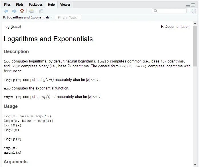
Datasets (DataFrames) and basic commands in R
R comes equipped with sample datasets that can be used to analyze and study data. For Instance the Iris dataset, which contains information on Iris plant. Moreover, it specifies measurements for four features measured for three variants of Iris flower (setosa, virginica, versicolor). All measurements are given in centimeters.
Calling the Iris Dataset
> irisSepal.Length Sepal.Width Petal.Length Petal.Width Species
1 5.1 3.5 1.4 0.2 setosa
2 4.9 3.0 1.4 0.2 setosa
3 4.7 3.2 1.3 0.2 setosa
4 4.6 3.1 1.5 0.2 setosa
5 5.0 3.6 1.4 0.2 setosa
6 5.4 3.9 1.7 0.4 setosa
7 4.6 3.4 1.4 0.3 setosa
8 5.0 3.4 1.5 0.2 setosa
9 4.4 2.9 1.4 0.2 setosa
10 4.9 3.1 1.5 0.1 setosa
11 5.4 3.7 1.5 0.2 setosa
12 4.8 3.4 1.6 0.2 setosa
Exploring Column Names in the Iris Dataset
> # Column names
> names(iris)
[1] “Sepal.Length” “Sepal.Width” “Petal.Length” “Petal.Width” “Species”
Returning an Object Deffinition for the Iris dataset
> # We usually work with objects of class data.frame, a table look-alike with columns and rows
> class(iris)
[1] “data.frame”
Returning the Dimensions of the Dataset with R Language
> # Dimension
> dim(iris)
[1] 150 5
Return First 6 Rows of a Dataset
> # First 6 rows of dataframe
> head(iris)
Sepal.Length Sepal.Width Petal.Length Petal.Width Species
1 5.1 3.5 1.4 0.2 setosa
2 4.9 3.0 1.4 0.2 setosa
3 4.7 3.2 1.3 0.2 setosa
4 4.6 3.1 1.5 0.2 setosa
5 5.0 3.6 1.4 0.2 setosa
6 5.4 3.9 1.7 0.4 setosa
Return a Specific Number of First Rows with R Language
> # Specifying number of first rows
> head(iris, 10)
Sepal.Length Sepal.Width Petal.Length Petal.Width Species
1 5.1 3.5 1.4 0.2 setosa
2 4.9 3.0 1.4 0.2 setosa
3 4.7 3.2 1.3 0.2 setosa
4 4.6 3.1 1.5 0.2 setosa
5 5.0 3.6 1.4 0.2 setosa
6 5.4 3.9 1.7 0.4 setosa
7 4.6 3.4 1.4 0.3 setosa
8 5.0 3.4 1.5 0.2 setosa
9 4.4 2.9 1.4 0.2 setosa
10 4.9 3.1 1.5 0.1 setosa
Return the Last 6 rows of a Dataset/DataFrame
This is a sort of a logical function. If the first six rows was head then this one is…
> # Last 6 rows of dataframe
> tail(iris)
Sepal.Length Sepal.Width Petal.Length Petal.Width Species
145 6.7 3.3 5.7 2.5 virginica
146 6.7 3.0 5.2 2.3 virginica
147 6.3 2.5 5.0 1.9 virginica
148 6.5 3.0 5.2 2.0 virginica
149 6.2 3.4 5.4 2.3 virginica
150 5.9 3.0 5.1 1.8 virginica
Return the Last 3 rows of a Dataset/DataFrame
In the same vein as the head example.
> # Specifying number of last rows
> tail(iris, 3)
Sepal.Length Sepal.Width Petal.Length Petal.Width Species
148 6.5 3.0 5.2 2.0 virginica
149 6.2 3.4 5.4 2.3 virginica
150 5.9 3.0 5.1 1.8 virginica
Descriptive statistics
Let’s look at the basic statistics commands like min, max, range, median, mode, standard deviation, and quantile. We can get them all by simply using the summary() function.
> # Show dataframe statistics
> summary(iris)
Sepal.Length Sepal.Width Petal.Length Petal.Width
Min. :4.300 Min. :2.000 Min. :1.000 Min. :0.100
1st Qu.:5.100 1st Qu.:2.800 1st Qu.:1.600 1st Qu.:0.300
Median :5.800 Median :3.000 Median :4.350 Median :1.300
Mean :5.843 Mean :3.057 Mean :3.758 Mean :1.199
3rd Qu.:6.400 3rd Qu.:3.300 3rd Qu.:5.100 3rd Qu.:1.800
Max. :7.900 Max. :4.400 Max. :6.900 Max. :2.500
Species
setosa :50
versicolor:50
virginica :50
Or we can examine them separately.
> min(iris$Sepal.Length)
[1] 4.3

> max(iris$Sepal.Length)
[1] 7.9

> range(iris$Sepal.Length)
[1] 4.3 7.9

> mean(iris$Sepal.Length)
[1] 5.843333

> median(iris$Sepal.Length)
[1] 5.8

> mode(iris$Sepal.Length)
[1] "numeric"

> sd(iris$Sepal.Length)
[1] 0.8280661

> quantile(iris$Sepal.Length)
  0%  25%  50%  75% 100%
 4.3  5.1  5.8  6.4  7.9
Plots: meet ggplot2, library for stunning graphics
R can plot data on its own, but the dedicated library you’ll really want to use is ggplot2. With ggplot2 you can create beautiful print quality and publication-ready data visualizations.
Ggplot2 is based on the grammar of graphics idea, which basically means each part of code stands for a component or a layer. As a result, we can add components together using +. The basic structure of any plot looks like this:
ggplot(data = , aes(x =, y = )) + geom_name()- ggplot(): creates an object and assigns columns from data dataframe to x and y axes
- geom_name(): plots the data in desired geometry, for example point, line, histogram, boxplot
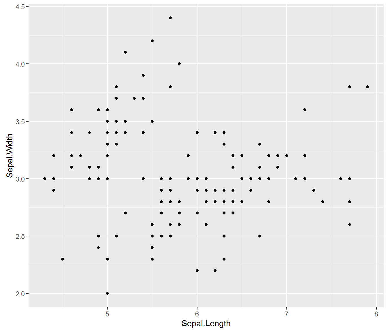
Point plot
Let’s plot a basic point plot.
We create a plot object using ggplot2, input the iris dataframe as data and assign the Sepal.Length column to x axis and Sepal.Width to y axis.
Further, add geom_point() to plot the points to the plot.
> library(ggplot2)
> ggplot(iris, aes(x = Sepal.Length, y = Sepal.Width)) + geom_point()
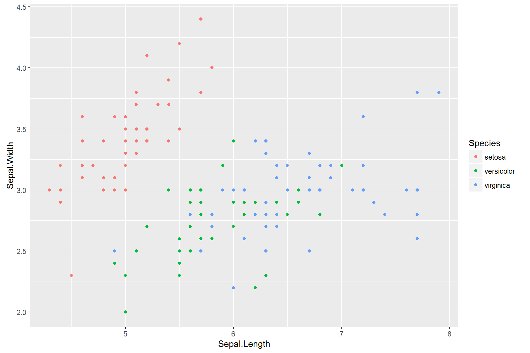
We often want to separate data according to the field in our data. We specify Species column as our color argument with color = Species.
> # Add colors to groups
> ggplot(iris, aes(x = Sepal.Length, y = Sepal.Width, colour = Species)) + geom_point()
Histogram in R Language
A histogram organizes a group of data points into ranges and plots the frequency of occurrence within each range. In short, this is the chart behind all normalized curves you will ever encounter. However, it should be said that for the best results while using a histogram settings will have to be manually adjusted most of the time.
> ggplot(iris, aes(x = Sepal.Length)) + geom_histogram()
To add color by group we specify Species column as our fill argument with fill = Species. For example, see the code below.
>  # Add colors to groups
> ggplot(iris, aes(x = Sepal.Length, fill = Species)) + geom_histogram()

Boxplot
Boxplot illustrates the distribution of data based on descriptive statistics: minimum, first quartile, median, third quartile, and maximum. In other words, it offers a lot of statistical information in one plot. Consequently, this is the chart of choice for a lot of Analysts and Statisticians.
> ggplot(iris, aes(x = Species, y = Sepal.Length)) +
	geom_boxplot()

Saving Plots as images or as PDF in R Language
Plots can be saved as images or PDFs directly in plot viewer by selecting Export > Save as Image or Save as PDF.

Alternatively, you can use function ggsave(filename, path). For example:
> ggsave(filename = "my_ggplot.png", path = "C:/temp")If the path argument is omitted, it will default to the current working directory.
Learn more about R Language
In conclusion, this was a quick overview of R basics. To learn more, stand by for our upcoming R Academy posts and Videos where we’ll go in-depth and cover all the relevant topics of R language.
Related Posts

- November 24, 2021
R Academy Menu ggplot2 basics: learn ggplot2 in 15 minutes!R ...

- November 20, 2021
R Academy Menu ggplot2 basics: learn ggplot2 in 15 minutes!R ...

- November 19, 2021
R Academy Menu ggplot2 basics: learn ggplot2 in 15 minutes!R ...
- November 12, 2021
R Academy Menu ggplot2 basics: learn ggplot2 in 15 minutes! R ...
Excel Unplugged acknowledgements


Donate
