R Beginner Tutorial – Matrices

In previous posts, we learned vectors and lists. Vectors are building block of other data structures. They can only contain one type of elements. Lists are similar to vectors but more versatile – they can contain all kinds of elements. A matrix however, can contain only one type of data. Matrices are similar to vectors in this regard.

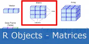
Let’s review how matrices compare to other data structures.

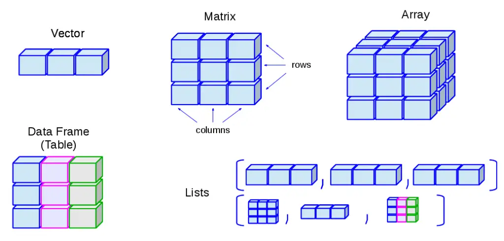
As seen on the image above, matrices can contain only one type of elements. Vectors, matrices and arrays must contain vectors of the same type, while data frames and lists can contain vectors of different types.

Let’s learn how to create and operate with matrices.

Creating a matrix

Create a matrix using matrix() command.

> # Elements are filled in by rows.
> m = matrix(c(1:12), nrow = 4, byrow = TRUE)
> m
     [,1] [,2] [,3]
[1,]    1    2    3
[2,]    4    5    6
[3,]    7    8    9
[4,]   10   11   12

> # Elements are filled in by column.
> m = matrix(c(1:12), nrow = 4, byrow = FALSE)
> m
     [,1] [,2] [,3]
[1,]    1    5    9
[2,]    2    6   10
[3,]    3    7   11
[4,]    4    8   12

Row and column names

Assign name to rows and columns with rownames() and colnames().

> # Define the column and row names.
> rownames = c("row1", "row2", "row3", "row4")
> colnames = c("col1", "col2", "col3") 
> m = matrix(c(1:12), nrow = 4, byrow = TRUE, dimnames = list(rownames, colnames))
> m
     col1 col2 col3
row1    1    2    3
row2    4    5    6
row3    7    8    9
row4   10   11   12

Accessing elements of a matrix

Access the element of a matrix by passing its row and column index m[i, j].

> # Define the column and row names.
> rownames = c("row1", "row2", "row3", "row4")
> colnames = c("col1", "col2", "col3")

> m = matrix(c(1:12), nrow = 4, byrow = TRUE, dimnames = list(rownames, colnames))
> m
     col1 col2 col3
row1    1    2    3
row2    4    5    6
row3    7    8    9
row4   10   11   12

> # Access the element at 1st row and 2nd column.
> m[1, 2]
[1] 2

> # Access the 2nd row.
> m[2,]
col1 col2 col3 
   4    5    6 

> # Access the 3rd column.
> m[,3]
row1 row2 row3 row4 
   3    6    9   12 

Matrix operations

Add, subtract, multiply and divide the matrices.

> # Create two 2x3 matrices.
> m1 = matrix(c(1, 2, 3, 4, 5, 6), nrow = 2)
> m1
     [,1] [,2] [,3]
[1,]    1    3    5
[2,]    2    4    6

> m2 = matrix(c(7, 8, 9, 10, -1, -2), nrow = 2)
> m2
     [,1] [,2] [,3]
[1,]    7    9   -1
[2,]    8   10   -2

> # Add the matrices.
> m3 = m1 + m2
> m3
     [,1] [,2] [,3]
[1,]    8   12    4
[2,]   10   14    4

> # Subtract the matrices.
> m3 = m1 - m2
> m3
     [,1] [,2] [,3]
[1,]   -6   -6    6
[2,]   -6   -6    8

> # Multiply the matrices.
> m3 = m1 * m2
> m3
     [,1] [,2] [,3]
[1,]    7   27   -5
[2,]   16   40  -12

> # Divide the matrices.
> m3 = m1 / m2
> m3
          [,1]      [,2] [,3]
[1,] 0.1428571 0.3333333   -5
[2,] 0.2500000 0.4000000   -3

In conclusion, this is how to operate with matrices. Next up, stay tuned and learn about arrays!

In a hurry?

Meanwhile, in a hurry? If you’re already running late, we recommend you head over to our two R crash courses:

• R Language overview, fast and easy beginner tutorial on R
• ggplot2 Basics, fast and easy beginner tutorial on plotting data in R

For even more amazing tips check out our awesome ExcelOlympics YouTube channel!

References

1 Ceballos, Maite and Nicolás Cardiel. 2013. “Data structure.” First Steps in R. Accessed 2021-10-12.