The Excel SEQUENCE function

In this article, we’ll introduce the SEQUENCE function. SEQUENCE function is one of the new dynamic arrays functions and when combined with other functions can do miracles! On top of its usual uses, most benefits can be gained from it when using the combination of SEQUENCE and various Date functions that can create dynamic calendars and dynamic YTD calendars. Also, the ability of transformations it offers is just amazing! But I’m getting ahead of myself. Let’s take a closer look at the basic syntax.

The sequence function syntax looks like this:

= SEQUENCE(rows, [columns], [start], [step])

Arguments are as follows:

• rows: number of rows
• columns (optional): number of columns
• start (optional): starting value of the sequence, with default value 1
• step (optional): step of the sequence, with default value 1

Before we dive in, let me just mention that we have a video on the Excel SEQUENCE function on our YouTube Channel and you can look at it here or at the bottom of this post. Thanks for your support!

Let’s look at a basic example. Type in the following formula.

= SEQUENCE(10)

Argument 10 defines the number of rows. The formula »spills over« rows and we get a column of 10 values. The default start is 1 and the default step of every sequence is 1.

The first argument defines a number of rows, but we can add a number of columns too. For example, 10 rows and three columns.

=SEQUENCE(10, 3)

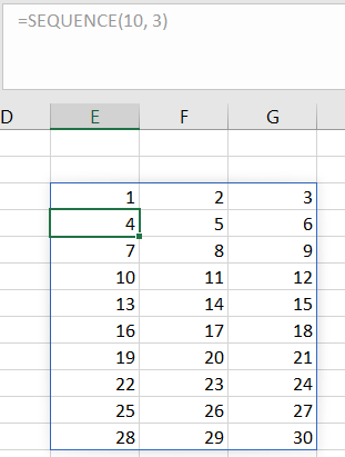
What we’ll notice is sequence fills the first row and the second and so forth.

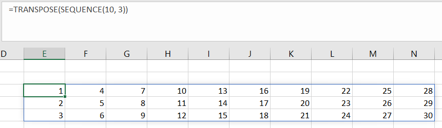
If we wanted the sequence to fill the column first, we could use the TRANSPOSE function.

= TRANSPOSE(SEQUENCE(10, 3))

Dates and the SEQUENCE function

We can now easily generate a sequence of dates using the SEQUENCE function combined with Date functions in Excel. We can get sequences of days, months, quarters, or Years.

A simple Sequence of Days

For example, let’s make a sequence of 10 dates starting with today’s date. Notice we left out the number of columns, which is 1 by default.

= SEQUENCE(10, , TODAY())

We now change the format to date.

Monthly sequences

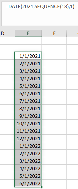
Or we can make a sequence of dates for the first day of the month. For example, for 18 months we would use the following formula.

= DATE(2021, SEQUENCE(18), 1)

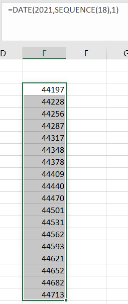
We again change the format to date.

Reporting sequence

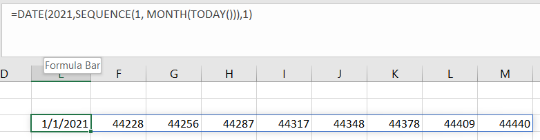
If we wanted a similar sequence, but for months leading up to today’s date, we would use the following formula.

= DATE(2021, SEQUENCE(1, MONTH(TODAY())), 1)

We then wrap the formula with the TEXT function to print out month names.

= TEXT(DATE(2021, SEQUENCE(1, MONTH(TODAY())), 1), “mmm”)

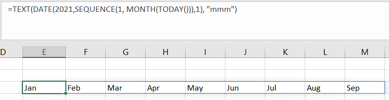
The great thing about this is, the use of the TODAY function makes it dynamic, so it will expand with time. By the time October rolls around, it will show October too! Reporting just got a lot easier.

Sorting values with the SEQUENCE function

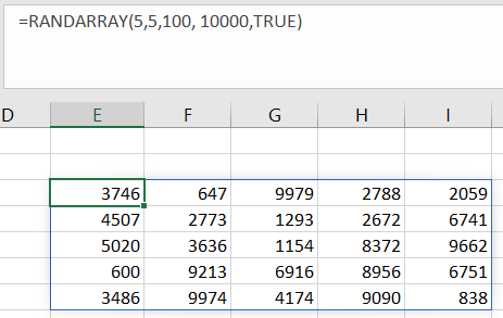
Another very useful trick is sorting values from a table. Let’s first generate a 5 x 5 table of random values between 100 and 10 000.

= RANDARRAY(5, 5, 100, 10000, TRUE)

Notice the TRUE argument for integer values.

We can now sort these values ascending or descending using the SEQUENCE function. First we create a sequence of the same length as the number of values, in our case 25.

= SEQUENCE(COUNT(E3#))

Next, we wrap this in Excels LARGE function.

=LARGE(E3#, SEQUENCE(COUNT(E3#)))

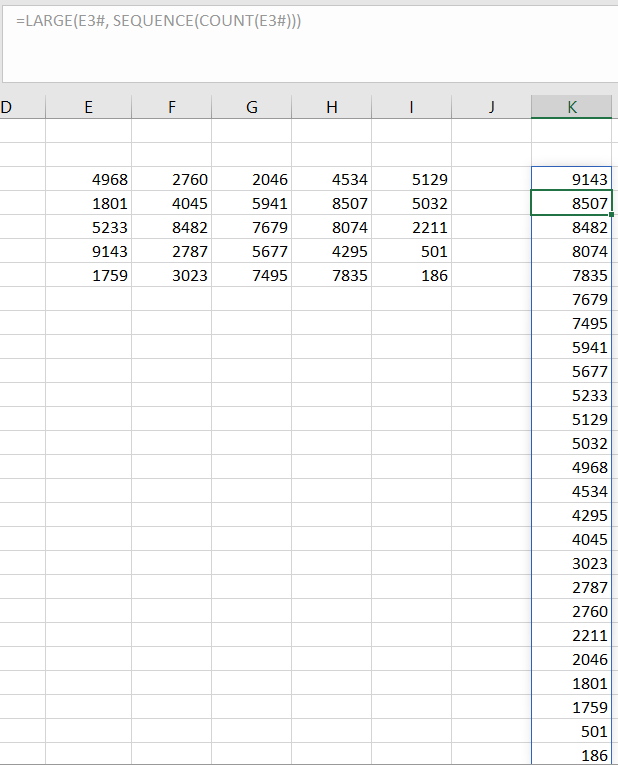
Voila, just brilliant!

Pivoting data using SEQUENCE function

Raw data often comes in the column form, and we then spread it out using different pivot transformations. Let’s look at how we can spread out data from a single column. (The data used is the sample data Ken Puls and I used in our session at the Bulgarian Excel Days. Have a look at that video (here) to see how you can “Pivot” data with Power Query)

We can quickly recognize a pattern of 7 rows that represent a single record. This means our data should have 7 columns. We create the following function.

= INDEX(A2:A50, SEQUENCE(7, 7))

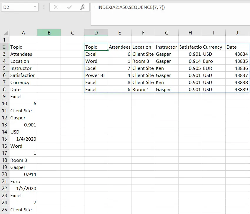
If only algebra was this easy!

Financial Modeling made easy with the SEQUENCE function

You could also use the SEQUENCE function in your models and have a dynamic or user-defined input. For example, we can define the possible input values using Data > Data Tools > Data Validation.

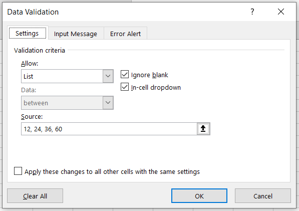
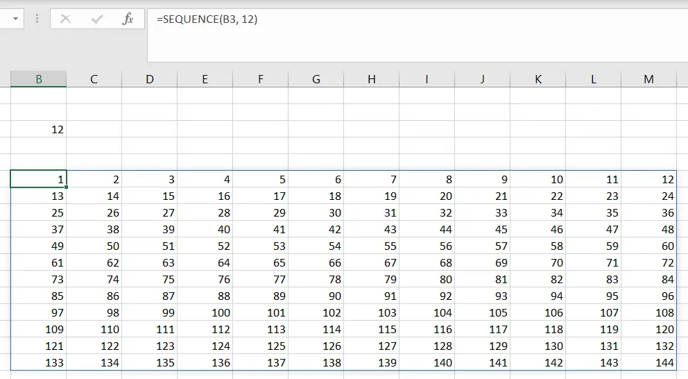
We’re allowing the user to select values 12, 24, 36, and 60. The default value is 12. We now enter a formula into another cell and use this user-defined input from the B3 cell as our argument.

= SEQUENCE(B3)

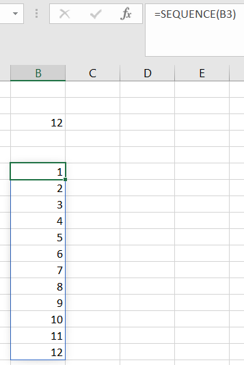
We get the entire sequence in one column. If we wanted a table instead, we add the number of columns, let’s say it’s also 12.

= SEQUENCE(B3, 12)

The user could now change the argument in cell B3 to 24. Our table will “automagically” grow!

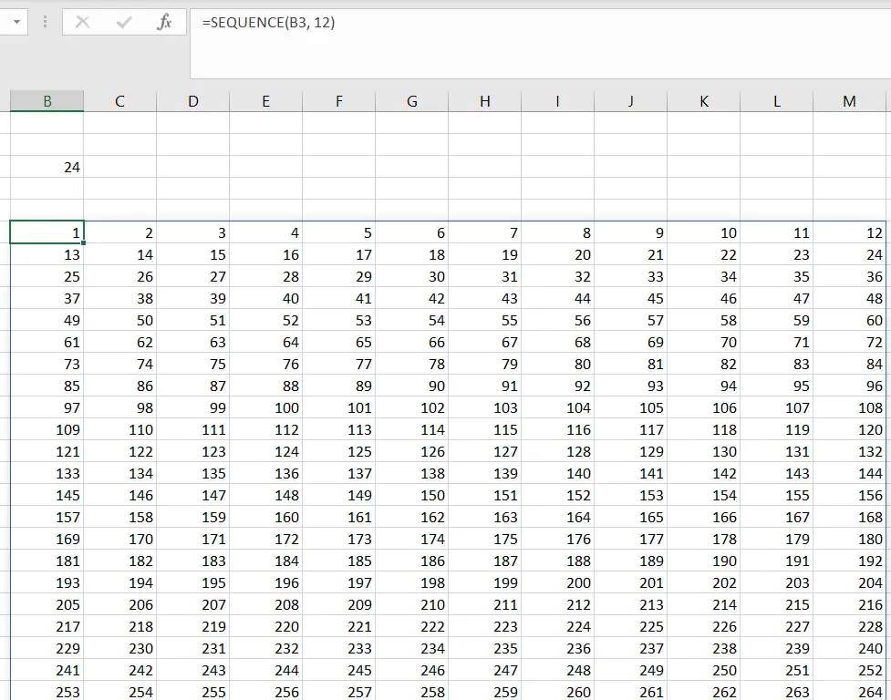
Just brilliant!

To see SEQUENCE function in action, watch our YouTube tutorial: