Excel FILTER Function – The Function that does Everything
- Gašper Kamenšek
- September 10, 2019
- 15 Comments

Last year, Microsoft announced the introduction of a new group of functions in Excel, known as dynamic array functions. One of these – the FILTER function – is possibly the best of the lot.
The FILTER function will filter a list and return the results that meet the criteria that you specify. This criteria can include multiple conditions and also AND/OR criteria.
Note: The dynamic array formulas are coming soon to Excel 365 subscribers only. Perpetual Excel 2019 license will not have dynamic arrays included.
What Makes this Function so Useful
The filter tool is one of the most useful features of Excel.
Sure, it may not be as flashy as Power Query, PivotTables and advanced formulas. But you watch Excel users at work, and everybody filters lists.
Well, we will now have filtering in the shape of a formula. Meaning it is automated, can return results to wherever you want them, and can be used in other formulas and Excel features.
Yes, you heard me right. The FILTER function could be used in a Data Validation rule or within a SUM function for a new and improved SUMIFS. Opportunities are boundless.
It can also be used as a supercharged lookup formula. Most Excel users are very familiar with VLOOKUP. It’s awesome!
However, it has limitations. Always looks in the first column, can only return one result, only tests the one criteria (without outside help).
The FILTER function (as you will see) can test multiple criteria, and from any column. It can return one (if looking for a unique value), but also multiple results.
Back in March 2018, Gašper wrote a brilliant two part article on Merge Queries being an alternative to VLOOKUP. Well, there is now a powerful formula alternative.
Excel FILTER Function Syntax
The FILTER function needs the following information to work.
Array – This is the range or array of values that you want filtered, and returned by the FILTER function.
Include – The criteria that you want to filter the range or array by. This can be any expression that results in TRUE/FALSE. The height of the range tested must be equal to the one provided in the array argument.
If_empty – An optional argument. This is the value to return if no records meet the given criteria.
Excel FILTER Function Examples
Let’s look at some examples of the FILTER function in action.
A Simple Filter
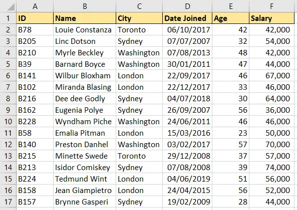
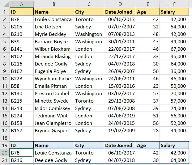
We will start with a simple text filter and filter the data below to only see the employees from Washington.
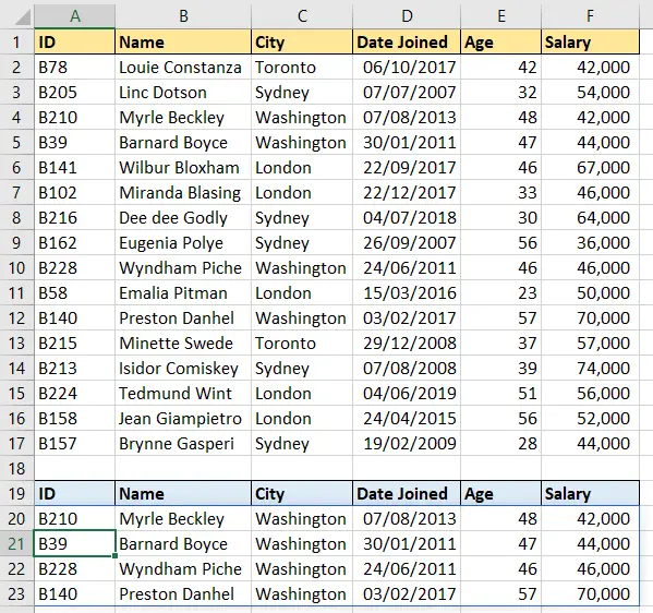
The following formula returns all columns of data if “Washington” is found in column C. Notice the height of the Array and Include range of equal.
=FILTER(A2:F17,C2:C17=”Washington”,”No results”)
The results are positioned under the data set here for better visuals for the article. Filter function can return the results to a different sheet or workbook, no problem.
Formula was entered into cell A20 but spilled into the range A20:F23.
The spill range is identified by a blue border.
This spill effect is a unique feature of the new dynamic array formulas. The formula only resides (and be edited) in cell A20, but its results spill to the array of cells outside.
If there was content in the area it needed to use, a SPILL error would be shown.
This is caused below by the 0 in cell E22.
However it is easily fixed by simply deleting or moving the naughty content.
If you make a mistake in the formula criteria such as a mistype on a city name. You will receive the CALC! error
No Ctrl + Shift + Enter
Advanced Excel users will have probably worked with array formulas before. They can be very useful, but can also be awkward to create, especially for the inexperienced.
One of the aspects of them that can make them awkward, is the need to press Ctrl + Shift + Enter to execute them.
Good news! The FILTER function can work with and produce a range of results without the need for Ctrl + Shift + Enter.
The VLOOKUP Alternative
I have mentioned how FILTER can be an alternative to the many uses of the ever popular VLOOKUP function.
Now this article would be mega if we went through all the possible cases, so let’s just see it performing a classic VLOOKUP scenario.
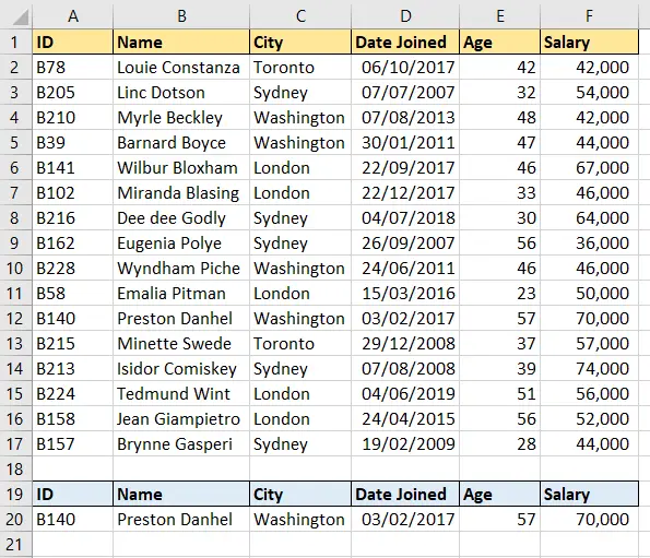
We would like to return the information for employee B140.
The following FILTER function is entered in cell B20.
=FILTER(B2:F17,A2:A17=A20,”No match”)
There are lots of take-aways from this example.
We can see the FILTER function returning information from columns B:F, but testing column A. So the criteria range does not need to be included in the returned range.
We are also testing a value from a cell (A20).
And final we have a built-in error response. If no value is found then the text “No match” is returned.
No IFNA or IFERROR functions needed.
With Aggregation Calculations
How about combining the FILTER function with an aggregation function such as SUM, COUNT or AVERAGE. That would be cool.
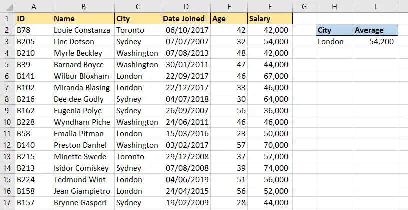
In this example, we will return the average salary for employees at the London office.
The following formula is entered in cell I3.
=AVERAGE(FILTER(F2:F17,C2:C17=H3,0))
The FILTER function returned the array of values from column F that met the criteria, and the AVERAGE function performed its task on them.
If no results are returned, the value of 0 is shown.
We rely so much on functions such as SUMIFS, COUNTIFS, SUMPRODUCT, AGGREGATE, VLOOKUP and the INDEX & MATCH combo.
And here we are seeing a new function with the ability to take on the tasks we have relied on these different functions for.
So far, we have only performed one logical test in the FILTER criteria. So, lets round this article off by exploring multiple conditional filters.
Multiple Criteria – AND Logic
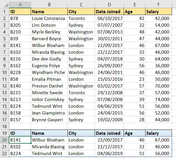
Let’s begin by using AND logic for two columns of data. We want to return the employees from the London office, who have joined since the 1st January 2017.
The following formula is entered into cell A20 to return 3 employees details.
=FILTER(A2:F17,(C2:C17=”London”)*(D2:D17>=DATE(2017,1,1)),”No results”)
The multiply operator (*) is used to perform AND logic tests, and each Boolean expression is enclosed in its own set of brackets.
If you have used array formulas or functions like SUMPRODUCT before, this approach will not be new. But here is a breakdown if your interested in how it works.
The two conditions are both evaluated resulting in True, and false for each employee.
=FILTER(A2:F17,
{FALSE;FALSE;FALSE;FALSE;TRUE;TRUE;FALSE;FALSE;FALSE;TRUE;FALSE;FALSE;FALSE;TRUE;TRUE;FALSE}*
{TRUE;FALSE;FALSE;FALSE;TRUE;TRUE;TRUE;FALSE;FALSE;FALSE;TRUE;FALSE;FALSE;TRUE;FALSE;FALSE}
,”No results”)
Two arrays containing the results of the conditions are then multiplied producing a 1 only where there is a True for both arrays.
=FILTER(A2:F17,{0;0;0;0;1;1;0;0;0;0;0;0;0;1;0;0},”No results”)
The 1’s represent the 3 employees returned by the FILTER function.
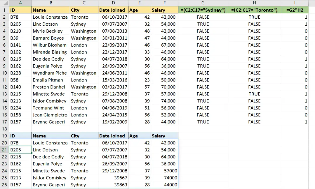
This is how it looks if we break it down into three separate calculations next to the data set.
You can include more than two conditions by continuing the same logic of surrounding each expression in its own brackets and using the multiply operator.
Multiple Criteria – OR Logic
OR logic can be used in the FILTER function in the same manner but using the plus operator (+) instead.
Let’s return the employees from both the Sydney and the Toronto offices.
=FILTER(A2:F17,(C2:C17=”Sydney”)+(C2:C17=”Toronto”),”No results”)
The breakdown from this is the same as before, however the two arrays are added to each other.
And this is how it works. But really just remember that you multiply for AND logic and add for Or logic.
You can also see in this example that the last few results do not have the correct formatting for the date and salary values. Although the dynamic formulas automatically spill into ranges, you will still need to format the cells just like with regular formulas.
Using AND and OR logic in the FILTER Function
Ok, let’s finish off by combining the two logics into one FILTER function.
We will combine the two examples we have done so far and return all employees from both the Sydney and Toronto offices whom started since the 1st January 2017.
=FILTER(A2:F17,((C2:C17=”Sydney”)+(C2:C17=”Toronto”))*(D2:D17>=DATE(2017,1,1)),”No results”)
Notice the OR logical test has been enclosed in another set of brackets here. This is important.
Remember the mathematical rules that multiplication takes priority over addition. Without the brackets around the OR logic, the formula would return the employees from Toronto who started since the 1st January 2017, and then all the Sydney employees.
=FILTER(A2:F17,(C2:C17=”Sydney”)+(C2:C17=”Toronto”)*(D2:D17>=DATE(2017,1,1)),”No results”)
It would fail to test the Sydney employees against the start date.
We would need to specify the OR logic first, then only the once since that start date.
=FILTER(A2:F17,((C2:C17=”Sydney”)+(C2:C17=”Toronto”))*(D2:D17>=DATE(2017,1,1)),”No results”)
The FILTER function is worth exploring further because it has huge potential to assist us in our Excel endeavours.
Especially when it is combined with the other dynamic array functions such as SORT and UNIQUE, and also existing functions as shown in this article such as AVERAGE.
Related Posts
- September 14, 2021
The Excel SEQUENCE function In this article, we’ll ...

