How to separate pivot tables in Excel? In this article we will discuss three different ways how to do this.

Why does Excel do this

During the creation of Office 2007, 2010 and 2013, a great emphasis was given to the file size. Of course you would like to make the file size as small as possible. For this purpose the creation or better yet the behavior of Pivot Tables has changed since Excel 2003. The Pivot Table has always created something called Data Cache based on the data provided. The need for indexing and fast creation of analysis has forced it to work in such a manner.

In Excel 2003 each Pivot Table had its own Data Cache, but now the Pivot Table that is created using the same Data Model or Data Source as another previously created Pivot Table also borrows that Pivot Tables Data Cache. Therefore, for each new PivotTable analysis that uses the “same” data, Excel saves hard disk space. It does not create its own Data Cache but rather uses the same one as previous Pivot Tables created on the basis of the same Data Model.

The problems it creates

While this solution is obviously a great way to save space on the computer, this also has two quite severe consequences for your Pivot Tables.

1.
Refreshing one individual Pivot Table consequently refreshes all Pivot Tables that are based on the same data, which can be a great thing but you can easily think of some cases where this would not be such a good thing.

2.
The grouping of records within a single field (for example, a Date field that you combine by months or quarters) now cannot be done on an individual PivotTable but immediately effects all the other PivotTables that are related to the same Data Model. If you used this field in another PivotTable, it reflects this grouping instantly. So you’ve lost the ability to group for example a Date field by months in one PivotTable and by Quarters in another.

How to change it

Both points listed above are reason enough for the need of a “separation” to arise. In fact, In this article we will discuss three different ways how to do this.

First way is linked to the creation of the new PivotTable report. It tells us how to create a PivotTable in such a way that it already has its own Data Cache and does not share one with the existing PivotTables.

Afterwards I will give you two methods on how to “separate” PivotTables that have already been created.

Method 1 (creating a separate Pivot Table report)

If you want to create a new PivotTable so that its Data Cache is separate from the other PivotTables you might have, then you must create it in a particular way. Better yet, create it with a special command called PivotTable and PivotChart Wizard. This command has been part of Excel for what seems an eternity, however since by default it is not on any of the ribbons, you have to add it to the Quick Access Toolbar. To do this, you go to File/Options, and then Quick Access Toolbar. Above choose Commands Not in the Ribbon

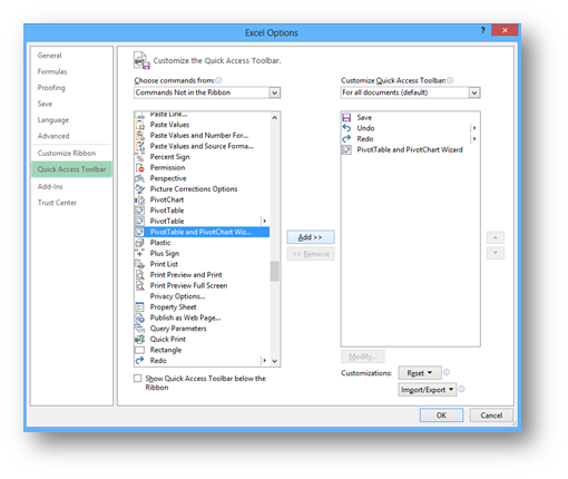
On the left side, find the Pivot Table and Pivot Chart Wizard and with the Add button add the commands to the Quick Access Toolbar.

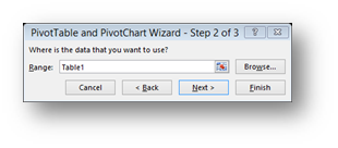
Afterwards we click in our data and run the command from the Quick Access Toolbar. This will sent us on a very familiar path 

The second one is very important, since it’s the step where we mark the area with the data for the the analysis.

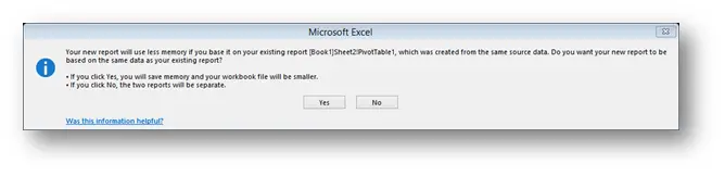
As soon as you say Next, get the following (important!) notice

If you select Yes, then the PivotTable will be calculated on the same Data Cache as preexisting Pivot Tables and it will suffer from all the symptoms described above. If you select No, then you will create a new Data Cache for this Pivot Table and therefor it will be separate from the preexisting Pivot Tables!

Method 2 (manual creation of a separate Data Cache for preexisting PivotTables)

The method is quite simple. Select the PivotTable that you would like to “branch off” and cut it from the workbook and paste it into a new one. Then you only have to copy the Pivot Table back to its original place. Sometimes this is enough. But sometimes, you have to close the first workbook and save the new workbook, close it, and then open both workbooks again and copy the PivotTable back into the original spot.

Method 3 (“separation” of already created PivotTables with the help of VBA code)

The following VBA code does the trick for all the PivotTables in your Workbook.

 Sub DataCache()

Dim PivTbl As PivotTable
Dim ws As Worksheet
Dim wsTemp As Worksheet
Dim pt As PivotTable

For Each ws In ActiveWorkbook.Worksheets

For Each PivTbl In ws.PivotTables

c = PivTbl.RowRange.Column
r = PivTbl.RowRange.Row
ws.Activate
Cells(r, c).Select
Set wsTemp = Worksheets.Add
ActiveWorkbook.PivotCaches.Create(SourceType:=xlDatabase, SourceData:=PivTbl.SourceData).CreatePivotTable TableDestination:=wsTemp.Range("A3"), TableName:="PivotTableTemp"
PivTbl.CacheIndex = wsTemp.PivotTables(1).CacheIndex
Application.DisplayAlerts = False
wsTemp.Delete
Application.DisplayAlerts = True
Set PivTbl = Nothing
Next PivTbl

Next ws

End Sub

And eternal happiness is even closer…

Learn more

Check out our YouTube channel and subscribe for more amazing Excel tricks!

Follow us on LinkedIn.

Check out our brand new R Academy!