One might think that analyzing data with a Pivot table is hard, but Unpivot a Pivot table proves to be even harder. But Power Query or better yet a Query editor proves once more that it is a brilliant tool that can handle Unpivot with ease.

Let’s first elaborate on what Unpivot means. From this

to this

Or in other words transforming a Pivot table back into a tabular and simply analyzable form. And It’s worth mentioning, it’s not limited to Pivot Tables, it can perform the same task on any two-dimensional data you have.

Now that we understand the problem, let’s get to it.

As the title suggests, a Power Query Add-In is required. Now personally, Power Query went from an Excel Add-In to a SWISS ARMY KNIFE excel tool and a MUST HAVE for every data cruncher out there. It’s free and you can get it here.

Now to begin the process, let’s start with the data table that looks like this.

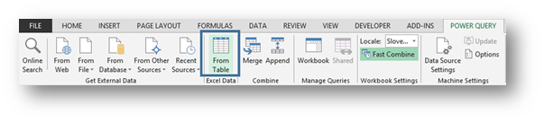
First item of business will be to take this data for a first spin in the Power Query Add-In. This is not a necessary step, but it will show you some beauty of the tool. So we select a cell that is part of the Table and go to Power Query/From Table

If this is the first time you’re using this tool it’s an absolute pleasure for me to present to you a window that will become your best friend in no time. Given the proper chance of course 🙂 . It’s called Query Editor.

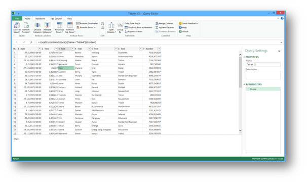
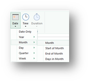
Now this is where the magic happens! If we want to do a pivot table summary like above, we will need year, quarter and month data in separate columns. All we need to do is to place ourselves in the Date column and go to the Add Column/Date/Year/Year command

And there it is

We repeat the process for Quarters and Months

And end up with

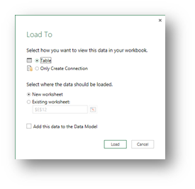
Again, we could have done the same in Excel by Year and Month functions and Quarters formula but this is much cleaner, easier and even more practical. If our initial table had many rows ( >500,000 ) then the amount of formulas written or calculations being performed would somewhat slow down Excel. But this way we get the calculation done and get it done dynamically! Let’s elaborate. Once the steps above are completed, we go to Home/Close&Load/Close&Load To…

And chose to load the result of this query into a new excel Table

Now this table comes packed with the Refresh feature…

And what this refresh does, it looks into the original Table and grabs any new data that may be there and then repeats the steps taken by the query, which were listed in the Applied steps list of the Query Editor. You can Edit this Query at any time and add or remove steps.

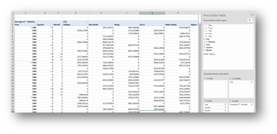
Creating the Pivot Table

The key with this pivot table is to have only one field in the Columns section and if there are more fields in the Rows section (in our case Year, QTR and Month), you should format the Pivot Table to a Tabular form and have the Item Labels repeated. The end result should resemble this.

And finally the Unpivot Query

Now that we created the Pivot table with the calculations we want, let’s “Unpivot it”. We go to a new Excel Workbook and from Power Query select From File/From Excel

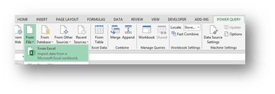
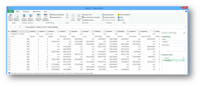
You then select a file and the Navigator lets you select the Sheet or Table you want to import. It even gives you a preview of the data.

Once the right Sheet is selected, you either select Load or the almighty Edit. If you want to Unpivot it has to be Edit, to get to the Query Editor. This will help us resolve all issues that would occur at a normal Pivot Table import.

1. The column headings are generic (Column1,Column2,…).
2. First row of data is obsolete.
3. The second row of data should be the header row.
4. Multiple “null” values where zeroes should be.
5. The Pivot shape.

Now we will tackle these problems one by one.

1. Remove Top Row

And then you must specify how many top rows you wish to remove. We will settle for just the one

And we get

1. Use First Row As Headers

And we get

1. Change “Null” into 0

Select all the columns where you wish to change a value and select Transform/Replace Values

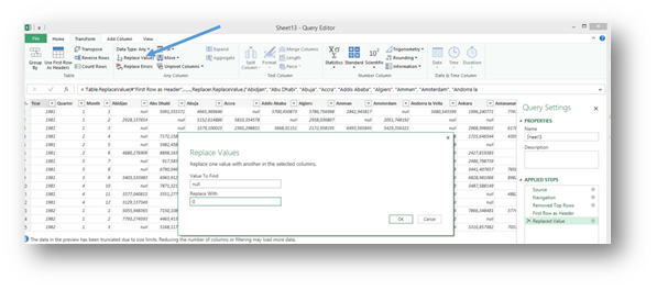
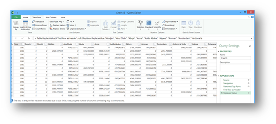
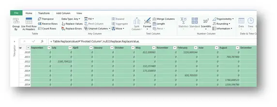
And you get

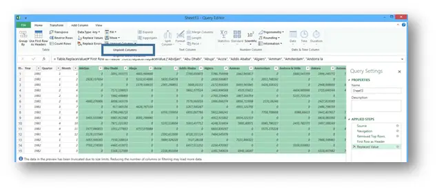
1. Unpivot

Now we select all the columns with the City names… So from Abidjan…to the last column and select Transform/Unpivot Columns

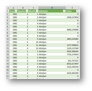
And here it is

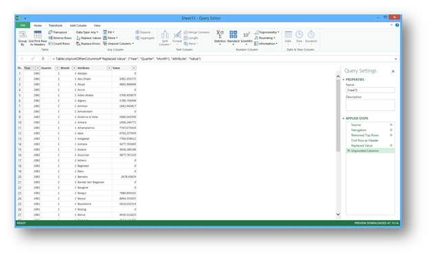
All the Pivot Table data in five columns 🙂 . The steps listed on the right can be individually edited or deleted. But after you select Home/Close&Load, you get a Table in Excel where you just right click and select Refresh and Excel or better yet Power Query will repeat all the steps for you and give you the latest data. I am confident, you can find many uses for this and I hope that it saves you as much time as it does for me.