Creating a dependent or linked Dropdown list
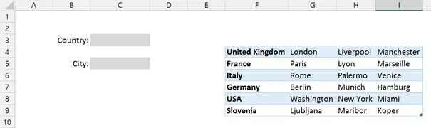
In this article I will show you how to create dependent Dropdown lists using Data Validation and an Excel function called INDIRECT. First let’s take a look at what we are trying to accomplish. We will start with the following workbook and data…
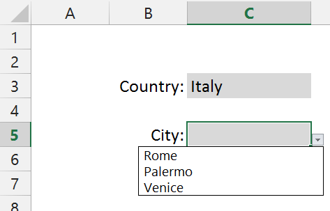
Now we wish to have two dropdown menus, one in cell C3 and one in cell C5. But, and here’s the catch, the dropdown in C5 has to be relative to whatever is choosen from the dropdown in C3. So if for instance someone picks France in C3, the dropdown menu in C5 has to give Paris, Lyon and Marseille, but if Slovenia is choosen in C3, Ljubljana, Maribor and Koper are in a dropdown in C5.
To achieve this we will use Data Validation with two additions. The first being the INDIRECT function and the second is using the named ranges.
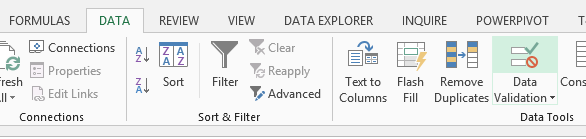
Just for clarification I will explain how to create a dropdown list in cell C3 using basic Data Validation. So standing on C3 you go to Data/Data Validation
In the dialog box you get you choose List under Allow: and point to the cells containing the names of the countries in the Source field.
So now you get a dropdown list in cell C3 where you can choose any of the countries.
It’s very important to understand that with using Data Validation to create the dropdown, and accepting all defaults under Error Alert you have also effectively limited the input into that table to only the values from the dropdown.
Before we can define the dropdown in C5, we must create a few named ranges so that Indirect will point to the right range.
We want to name the range where the French Cities are France and so on. We will use Excel to do this for us. We go to Formulas/Create From Selection and choose Left Column. So create the named ranges based on the values in the first column of the data I selected.
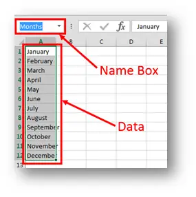
Doing this gives us six named ranges which we can see at the dropdown in the Name Box.
Pay extra attention to the United Kingdom name which was altered by Excel. The name reads United_Kingdom. The reason the underscore appeared is that names of ranges in Excel cannot include spaces. Therefor United Kingdom is not a valid name for Excel and it was changed. This will have dyer consequences for our sample but it will be a learning experience. So now that we have the named ranges we need, we can go to the next step but since the next step will include the Indirect function we should first familiarize ourselves with that function.
Just to clarify what the INDIRECT function does in Excel, here is a simple example of it in action (this is not part of what we wish to do, but just an explanationof the INDIRECT function). In A1 we have 100, in A2 we have A1. In A1 we write =INDIRECT(A2) and we get 100. So the cell that we give to the INDIRECT function actually tells the function where it should be looking. In effect, cell A2 told the INDIRECT function to go look into A1 and there it read the 100 it returned. Now we can really go to Step 3…
Same as in the above example, while standing on C5 we go to Data/Data Validation and say Allow: List. Now here the magic. Under Source: we write =INDIRECT($C$3) so we say to excel go and see what is written in C3. We already know it’s going to be a name of a Country. But with indirect we say go look at that name and see if there are any named ranges under that name. And INDIRECT tells the Data Validation which cells to take as a source and is effectively dependent on what is chosen in C3.
Now this works perfectly for all the countries except for UK, since cell C3 says United Kingdom, the named range for UK cities is under United_Kingdom (for reasons we discussed earlier) the INDIRECT function cannot work and produce a range for the dropdown.
In my next article I will be discussing the Named ranges or should I say Dynamic Named Ranges which can take this dropdown a level higher since it would be dynamic and you can add Cities and they dynamically appear in the Dropdown list.
And this is what we call eternal happiness
Probably the longest title of all times, but it leads to ...
Can you create a Data Validation Dropdown list that uses data ...
Our goal here, is to create a dropdown list by using Data ...
This site uses Akismet to reduce spam. Learn how your comment data is processed.
Hello,
Nice tutorial…I don’t suppose you know how to accomplish this (Dependent Drop Down List) when the source data is in a different Workbook?
thank you for a very interesting question.
This can be achieved. You open a workbook where you define a name just like we did in the post above. It is recommended that both the name of the range and the name of the workbook do not include spaces.
Now the problem you have is that in the Data Validation window you cannot name another workbook as a source for the dropdown list. But this can be overcome by first creating a named range in the same workbook where we want the dropdown. So Formulas/Name Manager/New and in “Refers To” you write ‘NameOfTheOpennedWorkbookWhereTheNamedListIs.xlsx’!NameOfTheRange
Do not forget, the source workbook must be opened when you are doing this!
This will give you a named range in the target workbook that is just the same as the one in the source but with one vital difference. This range can be referenced as a source for the DropDown List.
Hope this answers your question 🙂
Thanks for trying to help. I have tried that setup and it doesn’t seem to work for dependent drop down menus…works for a single drop down menu, but when when trying to get a dependent drop down situation with INDIRECT then only errors come back. At least that is the case for Excel 2011 on Mac. Anyway, ended up just having the data in a different worksheet in the same workbook and using tables (rather than INDIRECT) to set things up. Thanks again.
I’m trying to use this formula but it’s not working for me.
I’m trying to reference another file on my shared drive and it won’t let me begin a file name with a character. Could you provide an example from a file on a server?
Thanks
It doesn’t matter where the file is as long as it’s opened in Excel at the time you are referencing it in the Data Validation command. When you close that file, Excel will write down the full path needed for you.
You should look at my latest post
https://excelunplugged.com/2014/10/14/data-validation-dropdown-power-query/
it will give you a great idea how to use Power Query to achieve what you want.
I must tell you that it’s hard to find your posts in google, i found
this one on 18 spot, you should build some quality backlinks in order to rank your site, i know how to help you, just type in google – k2 seo tips and tricks
Hi,
Thank you for the comment, here are my thoughts on the matter.
First of all I must confess I know very little about Google and it’s search algorithms. But the reason I’m not concerned about the current search position of my pages is that the page and the ExcelUnplugged.com domain only exist since the 13th of May 2014. In addition, I still own an MS Excel Unplugged blog (gasperkamensek.wordpress.com) that most of the same content but is no longer maintained. I tried to tell google that the content was transferred but they said they couldn’t do anything since the gasperkamensek.wordpress.com is not an owned domain. So now I more or less just wait for Google to catch up. Every Tuesday I publish a new post so the content is getting bigger and as I see it sooner or later search results have to pick up…
Thanks for the help but for the time elapsed since the 13th of May, I think things are moving in the right direction.
Any idea how to link a table to a tab in a drop-down list? Pertaining to your example, I would want to display a table for Rome that shows monthly crime rates (for example), but then display a new table when I select Venice.
Hi,
this is the way I would go about doing this
https://excelunplugged.com/wp-content/uploads/2015/06/CHOOSE-tables.xlsx
It’s by using the CHOOSE function which you can see in action here. I think you’ve given me an idea what to write in my next weeks post 🙂
Hey hey!
Similar question to Travis’
I have a summary tab that has two drop down lists,
First drop down list contains months
Second drop list contains the names of worksheets (products) where data is pulled from a number of cells from the product worksheet (product values)
On those same worksheets, the dates have been grouped into months.
On the summary page which contains the two lists,
when a month is chosen, i’d like that to restrict the cells that the second drop down lists pulls data from
so that I can change the months, but still use the same product drop down list, while having update results if that makes sense.
Does the link in terms of your workbook post kind of deal with this?
Is there a way to copy this formula down? Ie; Using $C2 instead of $C$2? I am building a worksheet with accounts and then sub accounts using this method.
That will work… It certainly does in Excel 2016. Either by simply referencing a range or by using the INDIRECT method… Both approaches work.