Probably the longest title of all times, but it leads to something great. First let’s explain Power Query. Power Query is an AddInn for Excel and part of Microsoft’s Power BI (get it here). It is proving to be a tool Excel Users have been (unknowingly) waiting on for a very long time. This is a very simple use of that tool to achieve something that has so far been next to impossible to achieve.

The trick here is how to dynamically connect two Workbooks. So when you get new data in one, the other Workbook should result this growth (or shrinking) of data. We start this by having a Workbook called SourceDynamicRange.xlsx. On a Sheet called Data, a table called MyTable resides. It is very important that this is an Excel Table!

Now we go to another Workbook called DestinationDynamicRange.xlsx and there we go to Power Query tab and choose From File and From Excel.

As we point to our SourceDynamicRange.xlsx as an Excel file we wish to import, a list of all Sheets, Tables and Named Ranges (static names, not dynamic) is given. We choose MyTable. Also Notice a little preview of the selected data source which can be very useful in larger files.

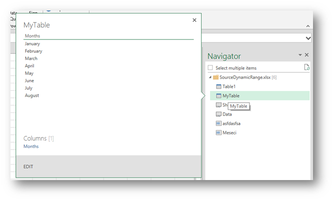
As we choose to import MyTable we get a new query and a table that is an exact replica of MyTable but resides in the DestinationDynamicRange.xlsx workbook.

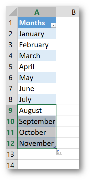
The best thing about it is, if we now choose to add data to our original table (the one called MyTable that resides in the SourceDynamicRange.xlsx). In this case I’m adding the next four months.

Save that file and go to the DestinationDynamicRange.xlsx, right click the replica table and choose Refresh (letting the query run again)…

There it is, eternal happiness.

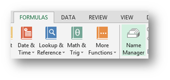
Now that this data is stored in this workbook, you can create a dynamic Named range. In this sample, you go to FORMULAS/Name Manager

Choose to create a new Named Range in my case I chose DynamicRange as a Name and in the Refers To you write

=OFFSET(Sheet9!$A$2,0,0,COUNTA(Sheet9!$A:$A)-1,1)

If you are interested in the OFFSET sunction and how the dynamic range written above works, read this article.

Now select the cell where you want your Data Validation dropdown and go to DATA/Data Validation

Choose List in the Allow dropdown and in the Source write “=” and the name of your dynamic range. In my case that is =DynamicRange

And there it is

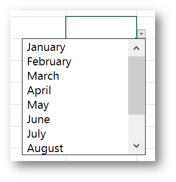
A Data Validation dropdown that is connected to a table in this workbook which is a dynamic replica of MyTable range in another workbook. Pure brilliance!

If you wish to read more about different (and more sofisticated) uses of Power Query, here are two articles you might find interesting:

Using Unpivot Column with Power Query

The new Pivot Column option in Power Query