Pragmatism vs. purity in Excel
- Gašper Kamenšek
- November 4, 2014
- 3 Comments

One of the greatest things about Excel is that with its endless array of tools and commands it almost always offers multiple ways of achieving a certain goal. Particularly lately with Excel 2013 with the new features that it brought not even mentioning the Add-ins it offers. In this array of numerous ways that one can go about doing things, knowledge is of course the first determining factor but after that, even with those that have the knowledge, there are some debates as to which way of doing things in Excel is better. Some Excel purists (particularly those that are familiar with Array formulas, will almost always opt in favor of formulas, whereas a pragmatic will always choose the fastest way (whatever it may be). I find this quiet battle very amusing and I guess the winners of the battle are always able to pick the better of the two approaches.
I will be showing both approaches on the following sample. From the data shown below we wish to extract only the numeric at the end. In other words, we wish to extract the last word in the string. Now I would urge you to look at both solutions for each may give you great ideas for your work in Excel.

Pragmatic solution
First we select the range of this strings by simply placing ourselves on any of the strings and pressing Ctrl + A. Then we will select the DATA/Text To Columns command.

Fist we select that our text is Delimited and press Next…

…and then tell the command that the delimiter is Space and that is followed by Finish.

Now we are a bit closer to our goal but still a far cry from it since the numbers we want are now spread through several columns. But all that’s missing is one magical move.
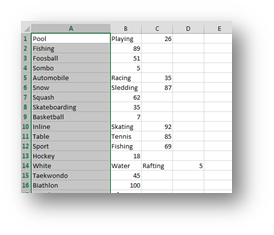
Again we do Ctrl + A, and press F5 or Ctrl + G. Select the Special button on the bottom left and choose Constants and text.

Now our selection looks like this.

Only one step left. Press Ctrl + – (control and a minus sign) and select Shift cells left.
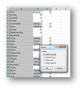
And we get
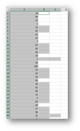
Eternal happiness.
Excel Purist
Now an Excel purist would do this

So the formula is
=MID(A1,MAX((–(MID(A1,ROW(INDIRECT(“1:”&LEN(A1))),1)=” “))*ROW(INDIRECT(“1:”&LEN(A1))))+1,50)
You must(!!!) enter this formula with a Ctrl+Shift+Enter combination (because it’s an Array formula) and excel will change it into
{ =MID(A1,MAX((–(MID(A1,ROW(INDIRECT(“1:”&LEN(A1))),1)=” “))*ROW(INDIRECT(“1:”&LEN(A1))))+1,50)}
As you can see, when we copy this formula down we get
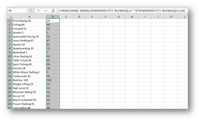
So exactly what we want but in a unique and elegant way. Keep in mind that this solution is slightly better than the first one since this formula can be edited, copied and reused. Next Tuesday I will explain this formula step by step… But for now, let it just stand, as a testament, to what can be done in excel and what may soon be obsolete since the arrival of Flash Fill in Excel 2013.
Flash Fill
Now I guess this is even more pragmatic than the solution above but it can only be achieved in Excel 2013!
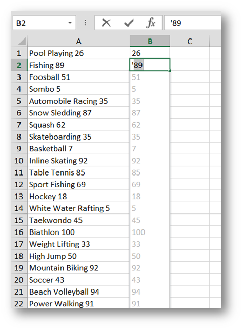
All you need to do is to rewrite the first number in the next cell. So we write the result we want in the first cell but with a twist. Since Excel knows that cell A1 contains text, the 26 in that cell is also regarded as text. That’s why we write ’26 in cell B1. So number 26 but stored as text.
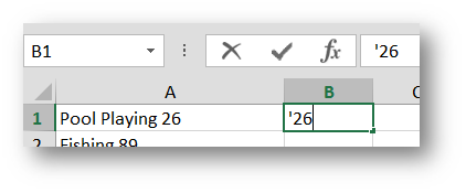
When you start writing the next number, as a matter of a fact, when you only input the ‘ sign, Excel recognizes your intentions and offers to help J. Just press enter and you’re home free.
With this three techniques under our belt, we can truly do amazing things in Excel.
Related Posts
- April 14, 2015
On February 3rd this year I published a post titled My Excel ...
- April 7, 2015
(as simple as Copy and Paste) This is our sample data. First we ...
- February 3, 2015
In my work as a Trainer and also as a Data Scientist (I love that ...


