The core of this blog post is a VBA code that will create a copy of a Power Query M code, modify it, create a new sheet and load the result of the modified Query to the new Sheet. This code was written and tested in Excel 2016. And if you want to follow along, here is a blank file to follow along.
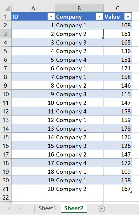
We will start with a simple Excel Table on Sheet2.
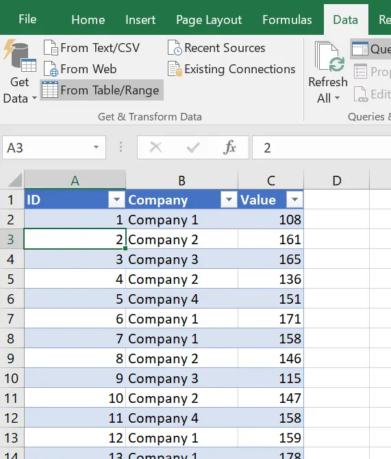
Now we create a Query that will read from our Table. We select a cell within the Table and go to Data/FromTable/Range
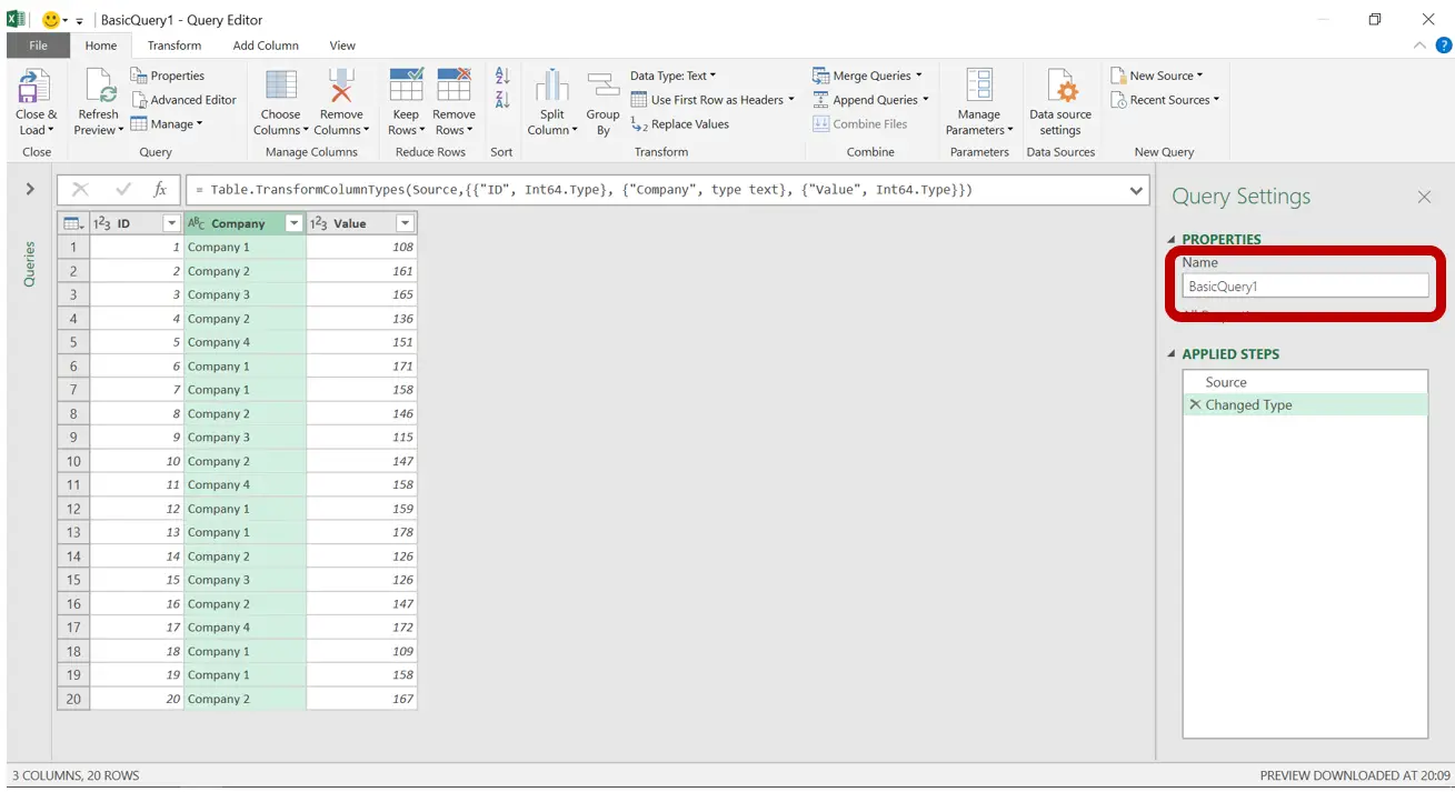
This will open a Query Editor. The first thing we want to do is to change the name of the Query in the Properties section of the Query Settings Sidebar. This is a very important step, as we need to feed the name into a VBA Input Box (you could also hard-code it into VBA but I wanted to make it dynamic). I called it BasicQuery1
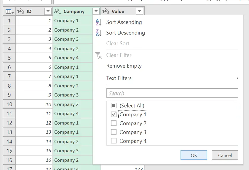
At this point we add an additional step to the query. In this step we will filter the Company column to keep only records of Company 1.
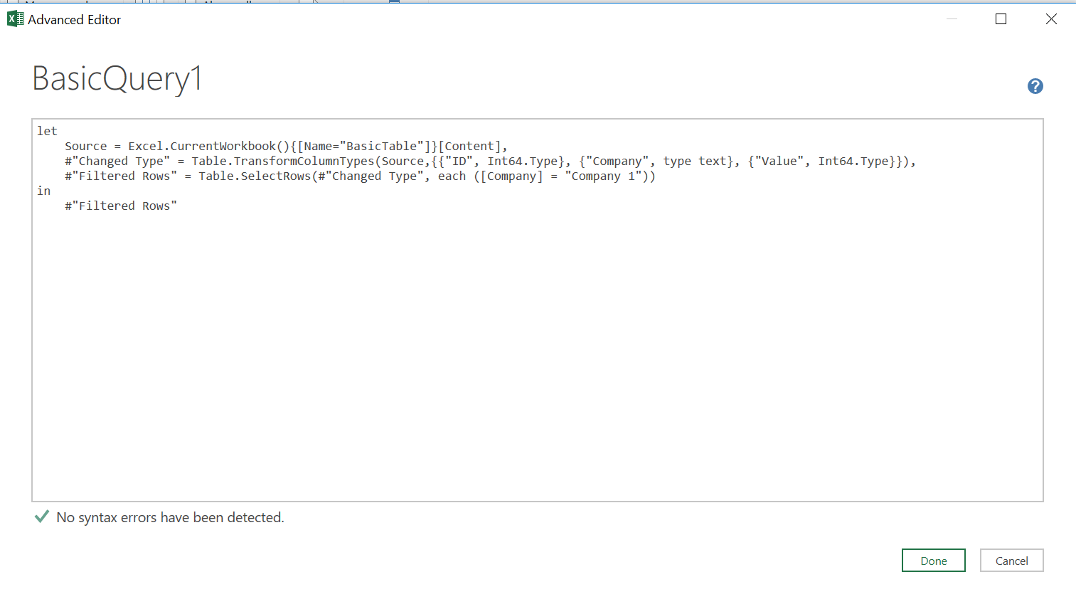
This step is the part of the Power Query M code that we will be changing with VBA. At this point if we choose the Advanced Editor command in Power Query Editor either on the Home tab or the View tab, we would see this
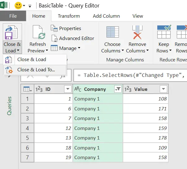
Now we’re finished with the Query and select Home/Close & Load dropdown and select Close and Load To…
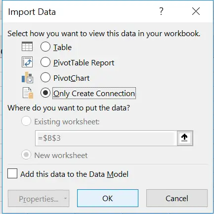
And we select Only Create Connection and OK
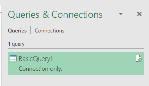
With this, Phase One is completed. Now we have our basic Query that we will modify with VBA.
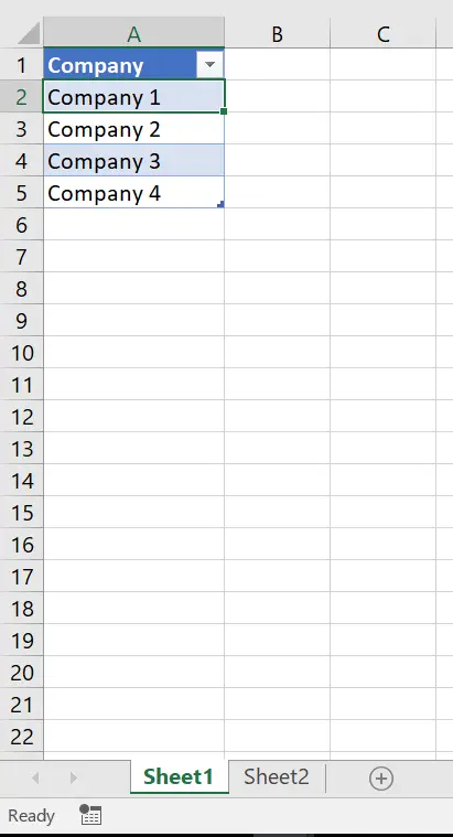
Now we get to Phase Two. We kick it off by creating an Excel Table with a list off all unique Companies from our original table.
We will step through this table with our VBA code and create a copy of our BasicQuery1 using these Companies as parameters for the final step (filtering of the Company column). We will also use the Company name for the name of the New Query and we will use it for the name of the newly created Worksheet where we will load the result of the Query. And now the VBA code:
Sub PQDynamicToSheets() Set aw = ActiveWorkbook Dim ws As Worksheet a = InputBox("Name Of The Basic Query?", "Query Name") '-----Read Basic Query Set q = aw.Queries(a) t = q.Formula '-----Read Filters Set tbl = Sheets("Sheet1").ListObjects(1) u = tbl.Range.Rows.Count - 1 '-----Go Baby Go For i = 1 To u '-----Current Filter nm = Sheets("Sheet1").Range("A" & i + 1).Value p = nm '-----UpdateQuery t1 = Replace(t, "Company 1", nm) '-----Create New Query p = aw.Queries.Add(p, t1) '-----Create A New Sheet To load Your Query Into Set ws = Sheets.Add(Before:=Worksheets(1)) ws.Name = nm '-----Change The Load Properties for New Query, so it loads on the new Sheet With ActiveSheet.ListObjects.Add(SourceType:=0, Source:= _ "OLEDB;Provider=Microsoft.Mashup.OleDb.1;Data Source=$Workbook$;Location=" & p & ";Extended Properties=""""" _ , Destination:=Range("$A$1")).QueryTable .CommandType = xlCmdSql .CommandText = Array("SELECT * FROM [" & p & "]") .RowNumbers = False .FillAdjacentFormulas = False .PreserveFormatting = True .RefreshOnFileOpen = False .BackgroundQuery = True .RefreshStyle = xlInsertDeleteCells .SavePassword = False .SaveData = True .AdjustColumnWidth = True .RefreshPeriod = 0 .PreserveColumnInfo = True .Refresh BackgroundQuery:=False End With Next i End Sub
The code revolves around the For statement. So, For each and every row in the first table on Sheet1, it remembers the Company name from that row and feeds it into the Update Query step which replaces the “Company 1” part of the query to whichever company was read from the current row. Once that is done, the next step of the code creates a new Sheet and names it after the currently selected Company. The last step just changes the load properties of the Query. Keep in mind, that our Query is just a copy of BasicQuery1 and as such it only creates a connection and does not load the result of the query. This final step changes the goal of the load to a Table on the newly created WorkSheet.
So as we run our code, we get this
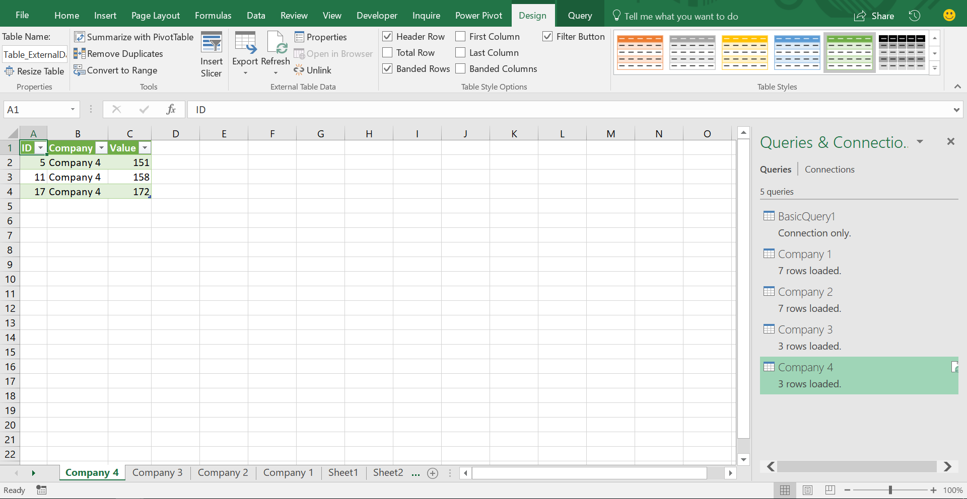
Four new Queries loaded to four new Sheets. Each with data just for that one Company.
In conclusion, this is how you modify Power Query M code with VBA. Eternal Happiness? We think so!
Check out our YouTube channel and subscribe for more amazing Excel tricks!
Follow us on LinkedIn.
Check out our brand new R Academy!
Let’s look at some crucial tools for creating polished ...
The Excel SEQUENCE function In this article, we’ll ...
Last year, Microsoft announced the introduction of a new group of ...
Today is most definitely one of the most exciting days of this ...
This site uses Akismet to reduce spam. Learn how your comment data is processed.
This is amazing! A combo of PQ (G&T), VBA & Pivot Table.
Could you also share your finished file?
@ Sandeep
Sure thing,you can download the file with the link below
https://excelunplugged.com/wp-content/uploads/2018/05/PQandVBA.xlsm
Great! Thanks.
Hi Gasper,
Even if, we have been talking a lot over several years in the Amsterdam Summit, I completely forgot about your blog.
This is a great article helping me in my Development for clients.
best regards
Jørgen
http://www.exceldoktor.dk
Hi Jørgen. Great to hear from you.
So now you will never forget about Excel Unplugged 🙂
Wow! realy mind blow solution.
It gave me of a possiable solution which I wanted to connect to web site in order to pull Rate of exchange BUT I want to keep the old ones as well, and not replace them with the new ones every time the query is running.
with your method I can make VBA code to copy, every time the query running, to summary rate of exchnage sheet.
Thanks!
Now some Web sites give you an XML pull of rates that includes history and is faster than a Web pull, but I am glad that this article helped you!
Hello! Your article seems close to what I’m looking for but not quite, and hopefully you can help 🙂
Let me start by outlining my current sheet/queries. My workbook has 6 queries in total, 5 of which generate tables, and 6 sheets with sheet1 being the raw data for the queries.
Steps
1. Paste raw data from a system report into a table in sheet1.
2. Connection only PQ sorts/renames/pretties up raw data.
3. PQ 1 filters a column and keeps only rows with a single value we’ll call “Value” the places it on a spreadsheet named “Value”
4. PQ 2-5 filters the same column, but to remove all rows with “Value”.
5. PQ 2-5 then adds an index column, then a calculated column “Number.Mod([Index],4) + 1”.
6. PQ 2 then filters all but “1” from the calculated column and deletes the Calculated and Index columns, PQ 3-5 does the same but with “2” “3” “4” respectively.
7. PQ 2-5 then output to separate worksheets named “1” “2” “3” “4”.
This has been working well until now, each table gets emailed to one of 4 groups to work on each day. My problem now is that we have switched to flexible teams, and some days it may be 3 teams others it may be 5, 6, etc. I am familiar with PQ and can just edit it manually, but this is clunky and most of my coworkers would not be able to do that. What I was trying to find was a VBA solution that would allow me to put buttons labeled “3” “4” etc on sheet1 that when clicked would generate the corresponding number of worksheets/tables and their power queries. The “Value” PQ never changes, and PQ 2-5 are identical with the exception of the value in the filter column step.
Does this sound possible, and if so would you know how to do it or be able to point me to a better resource? Thank you for your help!
I would think along the lines of putting a drop-down in Excel to select the number of groups and then naming that range (cell) and getting that value into Power Query via Excel.CurrentWorkbook() . I would then use this value as a parameter for the Mod and other functions previously using 4. Also making use of the {1..Parameter} to delete…
This is brilliant! Thanks a bunch for sharing.
Gašper,
Thanks for your work on this.
My company has just upgraded SQL Servers and now all my data sources (many XLSX & XLSM files with many, many queries per file) are hard referencing the old SQL Server. I thought about going the XML route to update but that seems fraught with danger.
I have already written the loop to go through all of my files by extension but how to update the query source seems to escape me:
Rough thoughts:
For Each qry In wrkbk.Queries
If Instr(qry.Source.String,”OLDSQLSERVERNAME”) > 0 Then
qry.NewSource.String = Sql.Databases(“”NEWSQLSERVERNAMEGOESHERE””),” & Chr(13) & “” & _
Chr(10) & ”
End If
Next
I have already copied and sandboxed my files to a backup drive so not worried about corruption testing this out.
Thanks,
Devin
Why even check if it has it, just do a “find and replace” with the VBA in the queries. If the old server name is not present, then nothing will change… But overall you are on the right track.
Thought I would post the code that worked for me; may help someone in the future:
“Sub FIXSQLREF()
For Each q In ThisWorkbook.Queries
If InStr(1, q.Formula, “OLD SERVER NAME”, 1) > 0 Then
q.Formula = Replace(q.Formula, “OLD SERVER NAME”, “NEW SERVER NAME”, , , vbTextCompare)
End If
Next q
End Sub”
This is so helpful! Thanks for putting it together!
Thank you Jeff for parts of your macro. I used it to list all the query’s in an Excel file
Sub list_m_code()
Dim lng_tel As Long
lng_tel = 2
Cells(1, 1).Value = “nr”
Cells(1, 2).Value = “name”
Cells(1, 3).Value = “M-code”
For Each q In ActiveWorkbook.Queries
Cells(lng_tel, 1).Value = lng_tel – 1
Cells(lng_tel, 2).Value = q.Name
Cells(lng_tel, 3).Value = q.Formula
lng_tel = lng_tel + 1
Next q
End Sub
Hello, is there a way to make the statement for “Company 1” dynamic in VBA?
Thanks
Sure thing, in VBA you can do whatever you want. I guess you would go through a column and create a list of unique values dynamically on each run…
Hi, I’m completely new in power query m language.
I’m trying to dynamically change the source. Doing this does not work:
formulaM = “let” & Chr(13) & “” & Chr(10) _
& ” Source = Web.Page(Web.Contents(“”” & ArrivalsTableLink & “””)),” & Chr(13) & “” & Chr(10) _
& ” Data0 = Source{0}[Data],” & Chr(13) & “” & Chr(10) _
& ” #””Changed Type”” = Table.TransformColumnTypes(Data0,{{“”Column1″”, type text}, {“”Column2″”, Int64.Type}, {“”Column3″”, type text}, {“”Column4″”, type text}, {“”Column5″”, type time}, {“”Column6″”, type time}, {“”Column7″”, type text}}),” & Chr(13) & “” & Chr(10) _
& ” #””Renamed Columns”” = Table.RenameColumns(#””Changed Type””,{{“”Column1″”, “”Airline””}, {“”Column2″”, “”Flight””}, {“”Column3″”, “”From””}, {“”Column4″”, “”Status””}, {“”Column5″”, “”Sched””}, {“”Column6″”, “”Updated””}, {“”Column7″”, “”Gate””}})” & Chr(13) & “” & Chr(10) _
& “in” & Chr(13) & “” & Chr(10) _
& ” #””Renamed Columns”””
Debug.Print formulaM
ActiveWorkbook.Queries(1).Formula = formulaq
If I pase the formula in advanced editor, it looks ok, but when refreshing error occurs.
How can I change the source?
Just open up your Query by double clicking it in the Query Sidebar and on the right go to the step called Source. You can change it here or you can have it reference a cell value…
Hello,
one question, code is very useful. It is possible before adding queries if there is no #Error in M code formula ?
I think you mean try… otherwise
Very helpful! I am interested to know if you also know a way to change the name of the connection itself when trying to clone an existing connection. I downloaded your template workbook and connection names are still listed as connection1,2,3,…so on. But I would like to refresh a particular connection on demand for which I need to give connections a specific name on the fly. Any thoughts?