Almost a year ago, more precisely in May of 2017 a site called defeat excel invited 27 Excel Experts (including myself) to end the endless debate of Vlookup vs. Index-Match combination once and for all. Needless to say, the goal was not achieved and to be fair, I think no one really took on the mission of a final count in that debate. Later as I was reading the contributions from others, I realised that the debate was totally pointless. And it wasn’t pointless only because everybody had their favourite picked in advance and just defended that one while realising both approaches had their pros and cons and confirming the fact that people would continue to use both just as they did before. No. The pointlessness of the debate came from the fact that at that point Power Query was already centre stage in Excel and could hands down beat them both!

The ultimate alternative I’m talking about in this post will not be an alternative function (or a combination of functions) but simply Power Query. And when I say alternative… What I really want to show in this post is that Power Query can do so much more than a simple Vlookup can.

In this week’s post we will be looking at three ways that Power Query builds upon the normal Vlookup and next week we’ll throw three more on the pile. And none of the six “add-ons” will be the lookup to the left because Vlookup can do that!

Ok first let’s set up a simple Vlookup scenario.

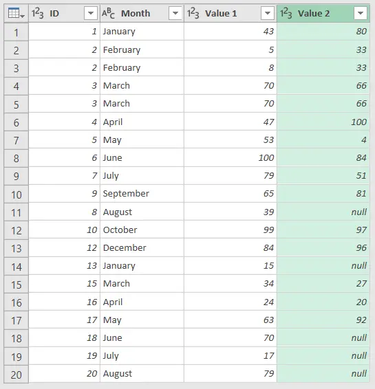
Two simple tables called Mother_Left and Lookup_right that can be matched by a combination of two columns, ID and Month.

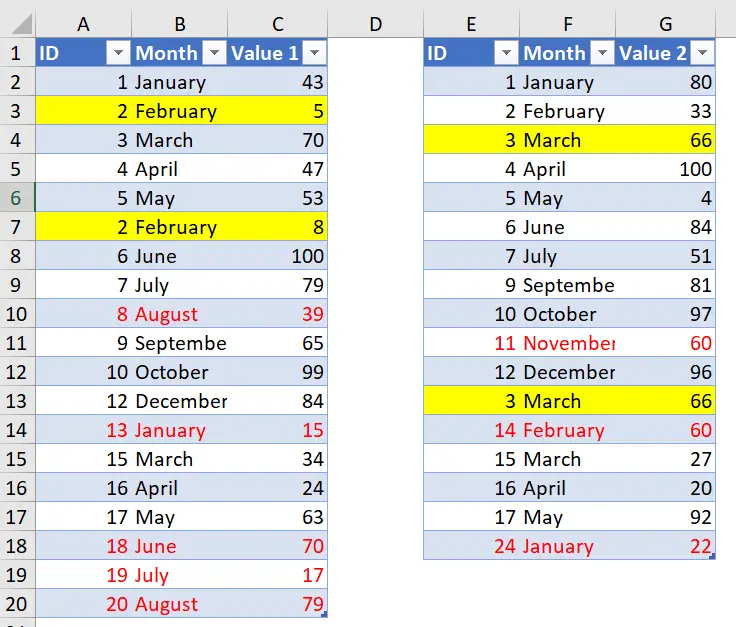
I’m sure you’ve noticed the best formatting practices (sarcasm!) to point out the things that Vlookup would not look kindly upon. The lovely yellow color (sarcasm again!) shows you duplicate rows in both tables. And the red font shows values that are unique to each table (they are not present in the other one).

First thing we should do is to set up two basic Queries which we will set up as connection only and will not load into the workbook. Those will serve as starting points for all our Vlookup queries in this post.

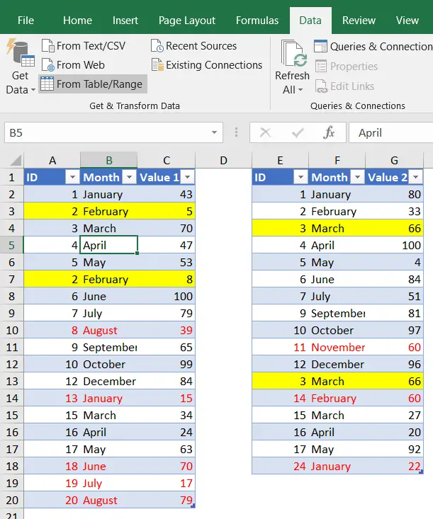
So we select a cell inside Mother_Left and choose Data/From Table/Range

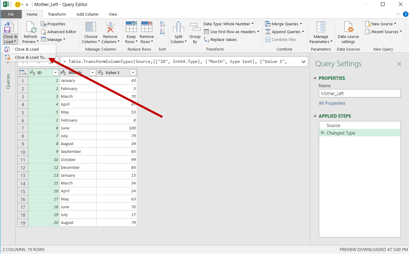
This will launch the Query Editor window where we simply select Close and Load To… from the Close and Load dropdown list.

And then choose Only Create Connection

After you repeat that for the Lookup_Right table, you should have this

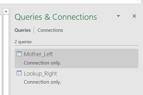
Both tables ready to go…

If you want the sample Workbook that already has all this steps and will serve as a basis for the Vlookup steps, you can get it here.

Now let’s start with the first Vlookup option you get with Power Query.

1      Matching by multiple criteria

I know that you can make Vlookup match by multiple criteria by making it an Array function and all that… But out of the box it just doesn’t do that. Here is how you make it happen with Power Query. After you have both tables accessible through Power Query, you select Data/Get Data/Combine Queries/Merge

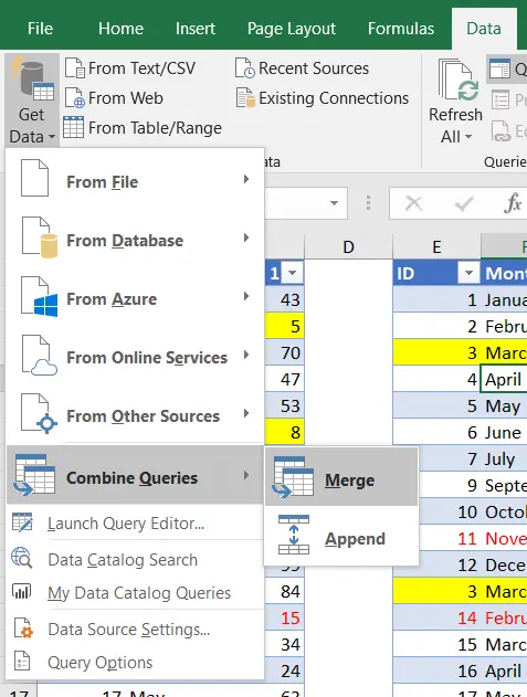
If you are using Excel 2013 or 2010 and have Power Query installed you choose Power Query/Combine/Merge.

The Merge Queries command is the starting point for all Vlookup equivalents and advances that we will show so memorize this procedure.

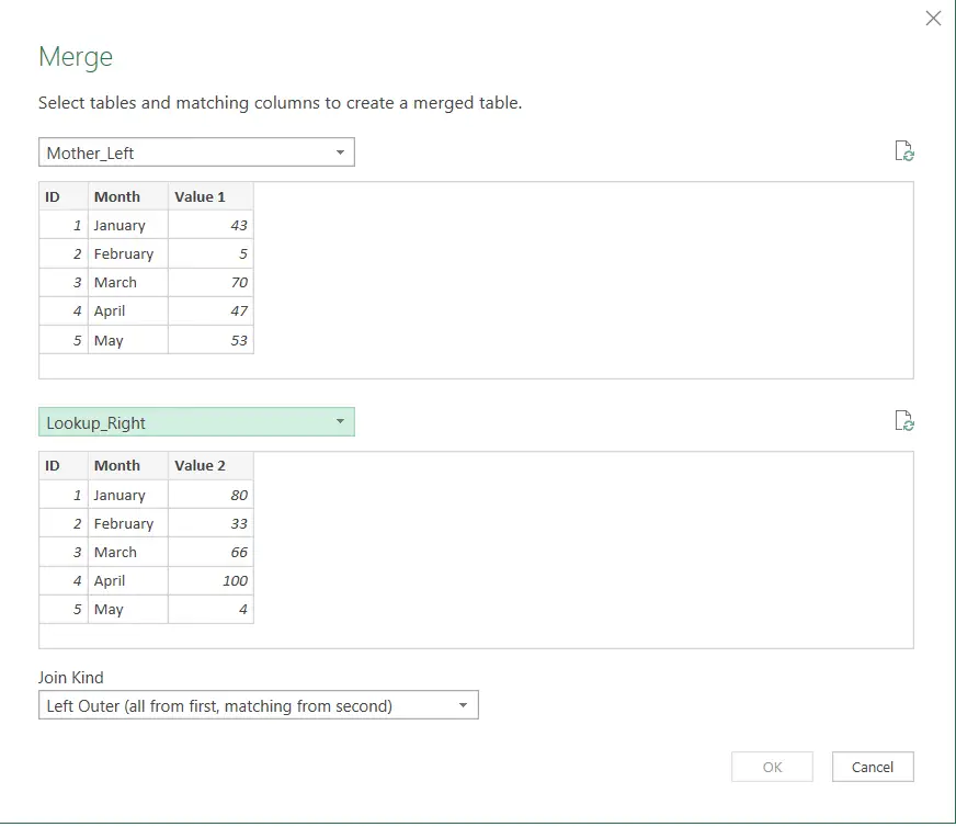
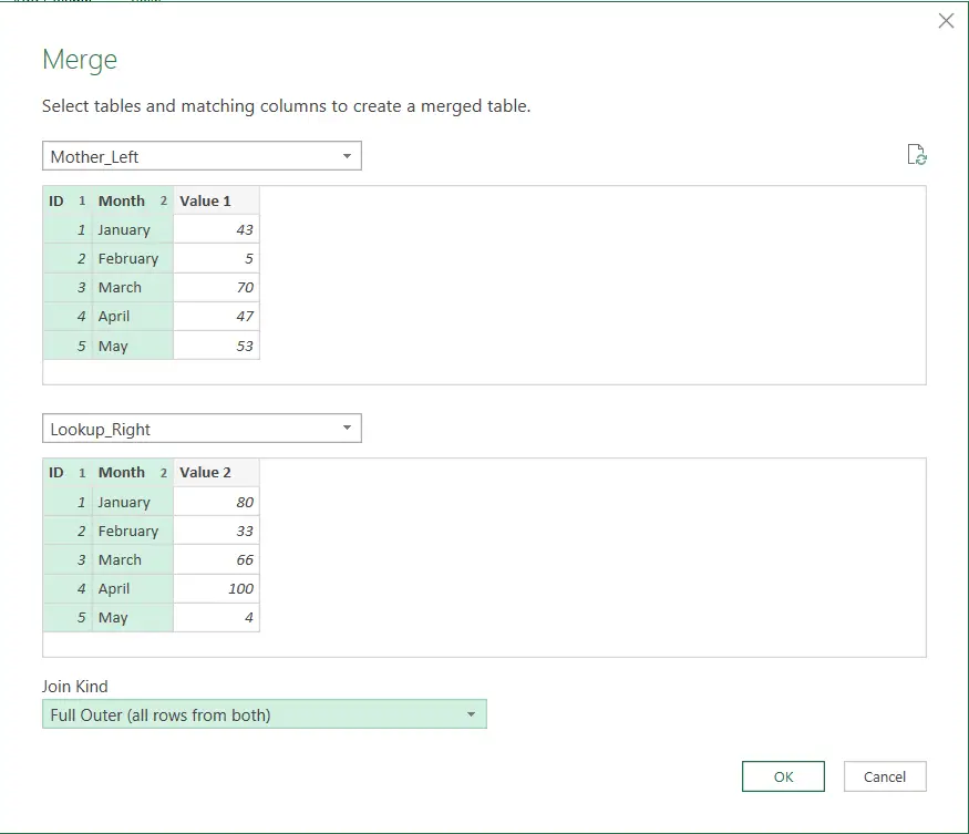
The Merge Window has three important sections that we will explain.

1. The dropdown in the top left corner enables us to select the Left table. That is the equivalent of the main table when you’re writing your Vlookups.
2. The dropdown in the top left corner of section two is where you choose your Right table (the lookup table).
3. This is where the magic happens. This is where you select “what kind of join” would you like to perform with the selected tables. Once again, this is where the magic happens.

The equivalent (but slightly better) of Vlookup as we know it in its function form is the Left Outer Join. It’s also the default selection for merging two tables and is the one we will use in our first example. After we select the Mother_Left in section one and Lookup_Right in section two, we get this.

Here comes the magic part… Selecting the columns to match by. You must do this for each table and if you want to match by more that one column, you select more columns as if you were selecting more columns in Excel. (By holding down the Ctrl key). After the selection, the Merge window should look like this

Notice the little numbers in the right side of the column headers. Those are extremely important! The names of the columns are totally irrelevant! It’s the sequence of selecting them that counts. And you should be true to your selection in the first table when you go and select columns in the lookup table. I hope you also noticed the sign at the bottom that informs you on how good the match will be. In our case it matched 14 out of 19 rows. What that means is that it found the desired combination of ID and Month in the lookup table for 14 of the 19 rows in the Main table. The ability to get notifications like this is amazing.

At this point we did all that we should do in the merge window and we should press OK.

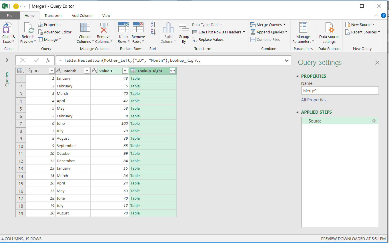
After you do so, you will once again find yourself in the Query Editor with all the rows from the main table and a new column reflecting the matched rows from the lookup table. This new column also has a special symbol to the right of the column header which indicates that this column contains more columns. All the columns from the lookup table to be exact! After you press the expand icon, you get to decide which columns from the second table to keep. Yes(!) you can select more that one at the same time ????

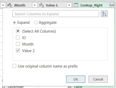
In the selection above I only chose to bring in the Value 2 column from the lookup table and I most certainly unticked the Use original column name as prefix, which is selected by default. After I pressed OK, I got this

A perfect Vlookup with a few extras! No errors where the value was not found (just empty cells (nulls)), and for ID = 3 and Month = March something even more amazing happened. It returned both(!) results from the Lookup table! Pure Brilliance!

2      Returning Non-Matching Values

This is probably one of the most amazing things that you can do with Power Query. The idea is to do a Lookup but only return things from the lookup table that you couldn’t find ????.

First let me say that if I wanted to return the rows from the Main table that didn’t get a match in the lookup table, that would be easy. Repeat all the steps from 1. Matching by multiple Criteria and filter for the null values, and that’s it. But we would like to get the values from the lookup table that obviously don’t exist in the Main table.

For this we repeat all the steps from 1. Up to the Merge window where the only difference from 1. Will be the Join type. The Join types that return non-matched values are the Anti-Joins.

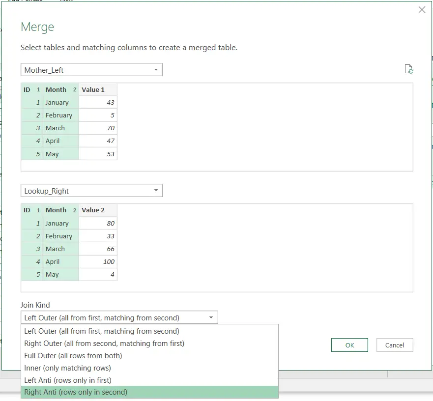
You can see both at the bottom of the dropdown list. The Left Anti Join would return the rows that only exist in the Main table. Put differently, the rows that have no matches in the lookup table. But to only get the rows that exist in the lookup table and have no matches in the Main table, you must select the Right Anti Join (as shown in the picture above). After you press OK, you get

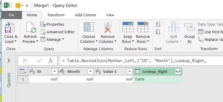
This we already recognize from 1. And after we expand the Lookup_Right column, keeping all the columns this time, we get this

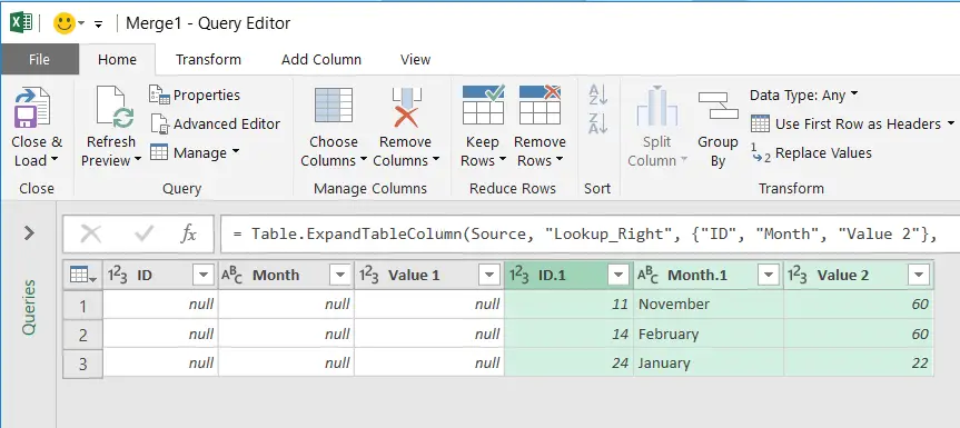
Now we’ve seen those rows before

There they are in red, indicating that they are unique to the lookup table. Now imagine that with Power Query you could potentially do this on tables coming from SQL, Oracle or any other system and the tables could contain millions of rows and by using Power Query you could quickly figure out which are missing from your logs… Or vice versa. Simply amazing!

3      Returning matching and Non-matching values

This will introduce a new type of Join. The Full Outer Join. Let’s just see what it does. So after repeating all the steps from 1., we select the Full Outer Join in the Merge window.

Press OK and we get this

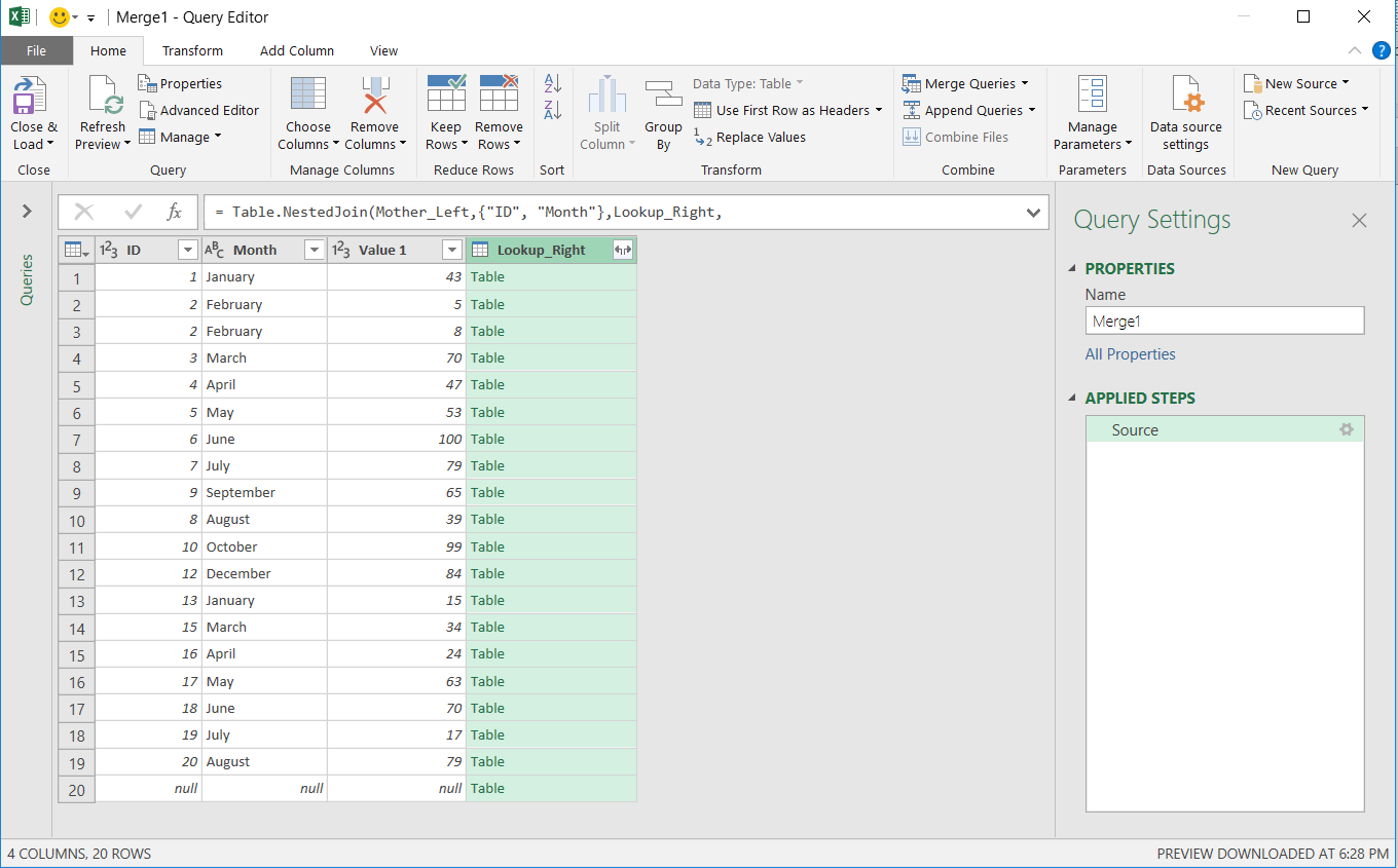
Ok, we know this already. We expand the Lookup_Right column and end up with this

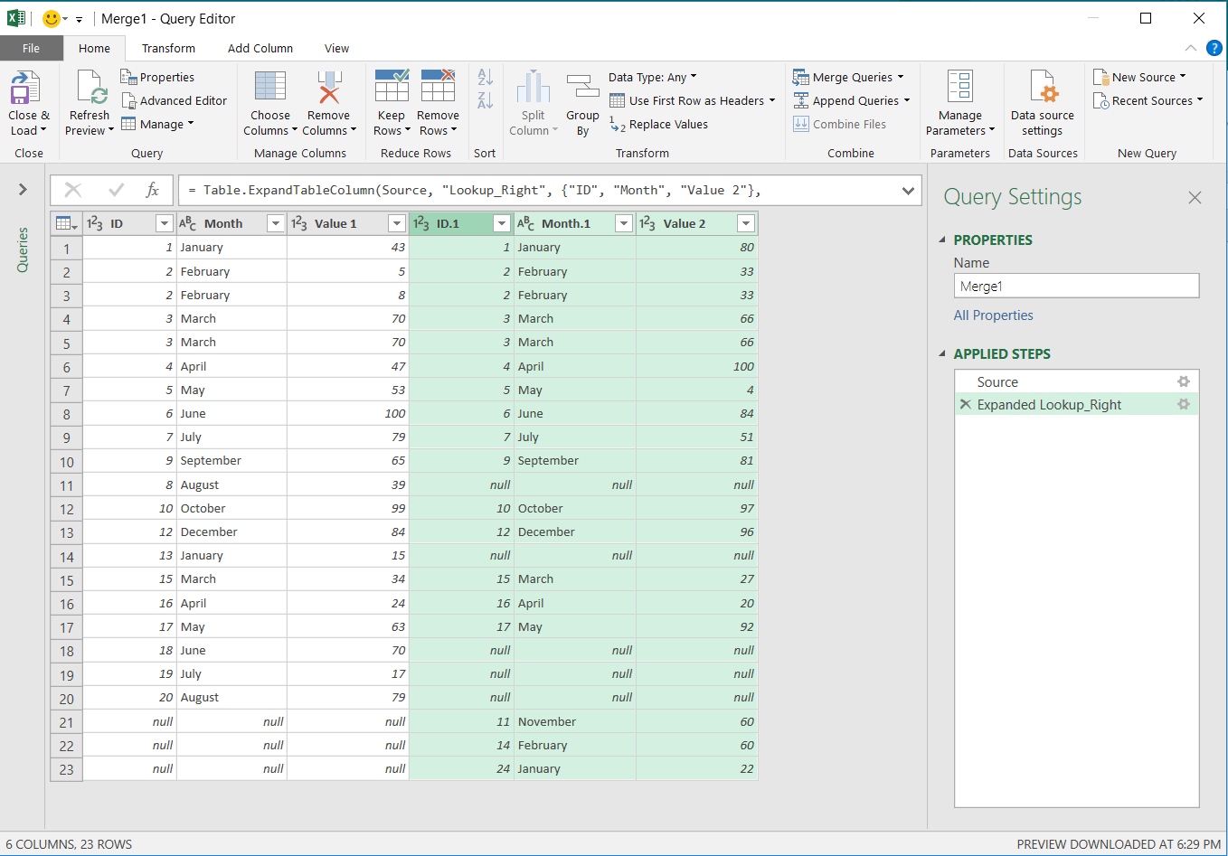
This one is a bit tricky but the main thing you should notice is that there are rows that have nothing but null values in the lookup table and in the end, there are rows that have nothing but nulls in the main table.

Now what is the result then?

It’s all the rows from the main table… Those that could be matched and those that couldn’t be. But on top of that you also get rows that are present only in the lookup table (they are not in the main table). So, you get all the rows from both tables and with a clear indication of which are only present in one of the tables. This is something that might as well have come from the Excel dream world it’s so good.

Read about three more incredible things that Power Query brings to the Vlookup table next week.