Increase your efficiency in Excel with these mouse based Excel shortcuts
- Gašper Kamenšek
- March 8, 2013
- 2 Comments

These days when talking about efficiency in any Office application, particularly in Excel, keyboard shortcuts are a must. But since we can’t really be efficient without the mouse, let’s see what are the hidden, but great uses of the mouse in Excel.
Paste as Value
Let’s start with one of my favorites. If you’ve opened Excel more than once, you have absolutely felt the need to copy some data and paste it as a Value (most commonly used when pasting data to a Sheet where the formulas would no longer function) . Where you only need the results of a formula but not the formula itself. My guess is that every Excel user goes about it the same way. Right click and Copy or Ctrl + C and then Right Click, Paste Special and I guess we all know the drill. But here’s another way to get the same result.
You select the Cell or a Range of Cells that you want to change to values. Then you place the mouse cursor anywhere on the edge of the selected Range but the bottom right corner. So anywhere but there! Now you right click and hold that click and then just shift focus, so swing the Range to the right (left, top, bottom) and back while holding the right click the whole time. When the active Range is where you want to Paste it, you simply release the Right Click. Then you will be condronted with the following menu in Excel…
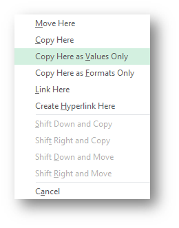
You select Copy Here as Values Only and here comes the eternal happiness we all seek 🙂
Fill Series
The Fill command on the HOME tab in Excel is home to some brilliant commands. Here are some great things it will let you do.
Create a Date Series of all weekdays in Excel (omits Saturdays and Sundays) – read about it here
Create a Factor Growing Series in Excel – read about it here
and my favourite (i bet you don’t know this one)
Fill and Justify in Excel – read about it here
But this will just tell jou how to get to the HOME/Fill/Series… command faster (with the mouse)
When faced with creating a series in Excel, we all turn to the Home tab and look for the Fill command. But here’s how the Excel pros do it…
Same as when using the Fill Series command, you write the first value in your series in a Cell and then place yourself on that cell. Next step is to place the mouse cursor in the bottom right corner of the cell’s border (so the exact opposite of the above example) and then Right Click, hold the click and again just shift focus (swing the Cell to the right (left, top, bottom) and back while holding the right click all this time). Now you get the following menu…
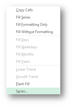
Some brilliant options there but the one we need is the bottom one Series…
Get around get around i get around
Borrowed the title from the Beach boys, but since Excel has 17,179,869,184 cells on one Sheet, it is vital that you can Get Around 🙂 The Ctrl + Arrows combinations are a given when maneuvering a large table. But the mouse can also get you there. It’s actually quite simple. You select a cell and if you want to go to the bottom of data in that column, all you have to do is place a mouse cursor on the bottom border of that cell, and then you just double click. If you placed yourself on the Right border, you would go to the last piece of data in that row and so on… As simple as that!
Related Posts
- April 14, 2015
On February 3rd this year I published a post titled My Excel ...
- April 7, 2015
(as simple as Copy and Paste) This is our sample data. First we ...
- February 3, 2015
In my work as a Trainer and also as a Data Scientist (I love that ...


