Boost your Excel efficiency with one key – F5 (Go To and Go To Special)

Very often you will find yourself in a position where you wish to either move efficiently through the workbook or you wish to select only cells containing certain kind of data (text, numbers, errors, objects, formulas…). The Go To… command which you get by either pressing F5, Ctrl + G or HOME/Find & Select/Go To… does it both. Let’s take a look at each functionality separately.

Moving through the Workbook
You probably know that you can move through and even select a range of cells in a workbook by using the Name Box, but there is a catch. If you make a mistake and write something that isn’t a valid cell address, Excel will (without warning) give the cell (or range) that is selected a name. Now this can be very useful but also a source of confusion. Here’s an example.

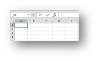
I’m in cell A1 and wish to go to E4. I will write _E4 in the Name Box by mistake and press enter.
Although Excel gives no warning, cell A1 was renamed to _E4.
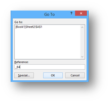
Now I will attempt the same with the Go To… command. So I press F5 and in the “Reference:” field I write _E4.
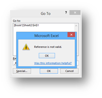
Press enter and something great happens, instead of renaming the active cell Excel warns me that the reference is not valid!
So a far more bulletproof method than the Name Box although it takes an extra key to get there :).
Defining or refining your selection (Go To Special)
Now this is pure magic in Excel. I will give four samples that will give you an idea of the usefulness here, but do feel obliged to explore this command further.
Example 1 (select only text):
Let’s say a very “evil” person did this:
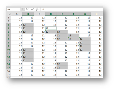
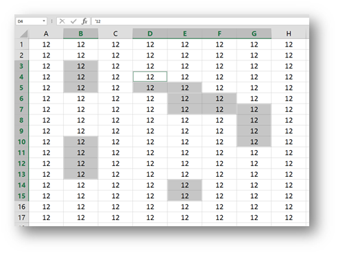
In a few cells a plain number 12 would be inserted, but in a few cells ’12 would be inserted. So a number 12 but as text.
Now at this point you can easily differentiate between the numbers and text but then the “evil” part 🙂
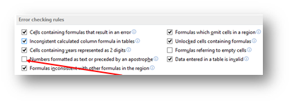
First we get rid of the error signs (green triangle indicators in the left top corner of the cell) by going to FILE/Options/Formulas and clear the check box next to Numbers formatted as text or preceded by an apostrophe.
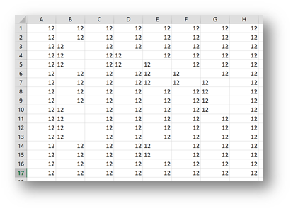
You can still see where the numbers are because of Excels default alignment but now that “evil” person gives all the cells Center alignment.
Now this could be a problem. We know some cells contain text, but it’s impossible to tell which ones. This is where Go To special comes in.
You can start by selecting all the data or by just standing in one cell. Then press F5 and in the Go To window select the “Special” button at the bottom left corner.
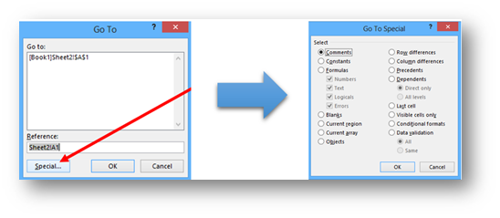
And here it is, one of the greatest Excel windows. As we wish to select the cells containing text, we will choose Constants (since all the data was inserted as souch, but we could also select formulas if we had calculations in those cells) and then only leave the check box next to text selected.

And voila, eternal happiness 🙂
You can chose only cells with Errors in the same manner or only Numbers… Definitely worth exploring.
Example 2 (select visible cells only):
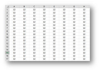
I used the same data as before but have hidden some rows (all that were in the way of true Fibonacci fans 🙂 ).

Now I wish to select the visible cells in column A to copy them to another sheet. So I select those cells by dragging from A1 to A13 and press Ctrl + C and then Ctrl + V n another Sheet.
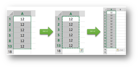
Oops?!? Weel I guess it can happen to anybody but how can we copy only visible cells? Since it’s impossible to guess I’m gonna tell you. It’s F5! So after you select the initial cells, you press F5 and press the Special button and select Visible Cells Only.

This gives you something comepletely different which you can see right away, but even better after you press Ctrl + C and paste the data.
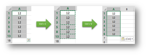
The difference (like the Chinese wall) can be seen from the moon 🙂
Example 3 (select objects):
Ever tried to copy a web page content to Excel? Let’s demonstrate with my daily stats of visits by country. After selecting all this data, I copy it to Excel.

This is what I get in Excel.

The data is OK, but I also got a number of flags that are only covering up the country names. So what I would like is to delete all the flags but to do that, I must first find the best way to select them all. You guessed it, it’s F5. So either while selecting the range of cells where the flags are or by just standing in one cell, we press F5, select Special and then Objects.

And we get

And just by pressing Delete, all the flags are gone.

As simple as that!
Example 4 (select blank cells):
This is the only example where you will want to start with the selection and then pressing F5 and choosing Special.

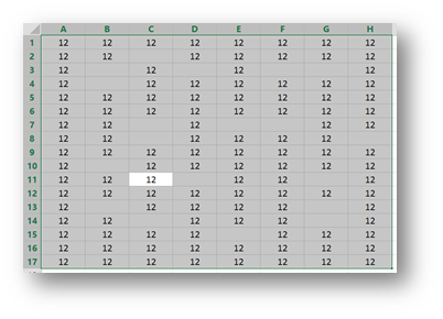
You select Blanks, press OK and you get

This combined with the Ctrl + Enter is truly a powerful weapon in Excel. Here is a sample of this and Ctrl + Enter in Action.
Now if you’ve read this article from start to finish I’m sure you got some great ideas where to use this new gained knowledge, and I assure you it will make you far more effective in Excel!
Tech Tip : Now get an easy one click access to all your essential Office 365 documents, data and windows applications on remotely accessible citrix xendesktop from CloudDesktopOnline with cheapest xendesktop pricing. To know more about Hosted SharePoint, Exchange and Office 365 visit www.Apps4Rent.com.
Related Posts
- November 30, 2021
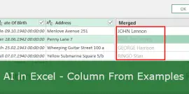
Welcome back to Artificial Intelligence in Excel! In Part 1, ...
- November 2, 2021
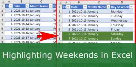
Highlighting Weekends can be hard in Excel. So just for fun, ...

- September 14, 2021
The Excel SEQUENCE function In this article, we’ll ...

- September 10, 2019
Last year, Microsoft announced the introduction of a new group of ...
Excel Unplugged acknowledgements


Donate
