Get a random subset of data with Power Query
- Gašper Kamenšek
- February 14, 2017
- 0 Comments
How to get a random subset of data with Power Query? The other day I made a Dashboard with a classic by time and relevant dimensions analysis. The data was pulled from Azure SQL DB, so Power Query was the method I used, to get the data into Excel. The dashboard build was very straightforward, until the customer desired to see a whole section that would show a “Random” analysis or rather analysis by random conditions. Sort of an element of surprise on the dashboard.
With that in mind I jumped right into the “random” side of Power Query, since my goal was to only import a random subset of data. This post will take you through the process of creating a query that will return a random subset of a table in a different workbook.
Here is the file I’ll be using, if you want to follow along.
Prepare BasicData table
We will take data from a simple Excel Table called factTbl, that looks like this…
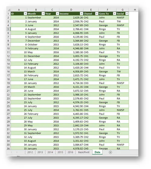
…and we want the “random” part of the analysis to focus on a random value of the “Goes To” column. So basically, all the rows belonging to One of the Fab Four J.
We start with a blank Excel File and go to
Excel 2016:
Data/New Query/From File/From Workbook
Excel 2010 or 2013:
Power Query/From File/From Excel
Select the desired file, and the right table and choose Edit

At this point you should see something similar to this.

Now we should rename the last step, so it will be easier for us to recall it later. We do this simply by right clicking on the step name (Changed Type) and selecting Rename.

I’ll name it BasicData. You can call it anything you want (if the name is not already in use), but make it sensible, so you can refer to it any time.
Remove the columns and duplicate values
Now we are ready to plant that random seed J
First we should remove all other columns, except for the “Goes To” column. Right click the “Goes To” column header and select Remove Other Columns.
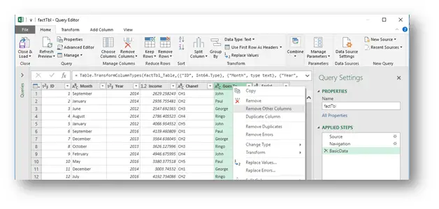
Next up, we remove all the duplicate values from the “Goes To” column. Same procedure, right click the column header and select Remove Duplicates.

Write the function
Now, we start writing a function that will select a random Beatle J.
Click the fx icon in the Formula Bar, leave the automatic formula as is, and just add [Goes To]{0} at the end.
If you did everything by the book, you got
= #"Removed Duplicates"[Goes To]{0}

What that essentially means is: “Based on a result of the “Removed Duplicates” step (that is the “table” we are working with), go to the “Goes To” column and return the first (!!!) element. Power Query is 0 based so “0” means “one” or rather “first”.
Now you can play around with this, by substituting the 0 by any other number up to three. And you will get the corresponding Beatle. But the trick is, how to make that number random. Therefore, we need a sort of RANDBETWEEEN (Excel) function in Power Query. The Power Query equivalents of Excel functions are:
| Excel Function | Power Query Function |
| =RAND() | =Number.Random() |
| =RANDBETWEEN(min,max) | =Number.RandomBetween(min,max) |
But there is a catch! The Rand and Number.Random functions are equivalent and work basically the same, but the Number.RandomBetween function on the other hand, does NOT work like the RANDBETWEEN function in Excel. The Excel version returns a whole (!!!) number between desired min and max values, but the Power Query version returns a random decimal number between min and max values.
So to use that function instead of a {0} in our function, we need to round it up to a whole number. And to get the equal representation of all numbers, we will use the following.
Number.RoundDown(Number.RandomBetween(0,3.99))
After replacing the 0 above with the function above, we get this:
= #"Removed Duplicates"[Goes To]{Number.RoundDown(Number.RandomBetween(0,3.99))}
Remark: Since we know there will never be another Beatle, the top can be a constant (3.99), but realistically we should add a row count of the table of all unique’s to the query, to make the top dynamic. The function we would use to count the number of rows would be = Table.RowCount(#”Sorted Rows”)
Refresh Preview
Now go wild with the Refresh button and you will see, that you do get a random Beatle…

This is our magical step that will give us that randomness. To make the reuse of this result as simple as we can, we should rename this last step into something more sensible. I’ll rename it to Beatle.

Call and edit the BasicData table
Now let’s call back our original table. Click the fx icon in the Formula Bar and call back the name you gave the original table (in my case that is BasicData).
=BasicData

Now we set up the filter that we need. So select the filter in the “Goes To” column and filter out your favorite Beatle.

With this we created a formula that only needs a little tweak…

…all that remains is to change the constant “John” (in my case) with our random variable Beatle (in my case, you might have used a different name).

Refresh, close and load
Once again go wild with the Refresh button J
At this point you can try and create more filters by other columns and add some more randomness to your result.
But to bring this post home, just Close & Load…

…the data into Excel and then if you so desire, you can go wild with Refreshing the Query.

One step closer to eternal happiness yet again J
Learn more
Check out our YouTube channel and subscribe for more amazing Excel tricks!
Follow us on LinkedIn.
Check out our brand new R Academy!
Related Posts
- November 9, 2021
Let’s look at some crucial tools for creating polished ...
- September 14, 2021
The Excel SEQUENCE function In this article, we’ll ...
- September 10, 2019
Last year, Microsoft announced the introduction of a new group of ...
- August 28, 2019
Today is most definitely one of the most exciting days of this ...

