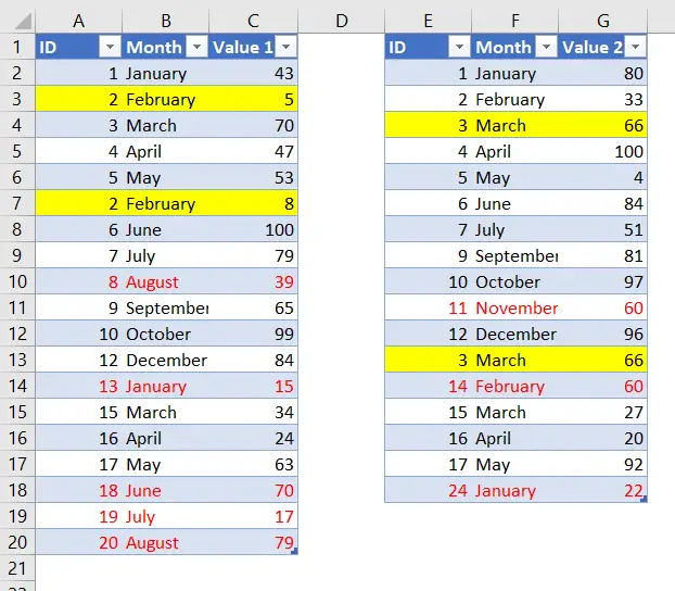
This is part 2 of the Ultimate Vlookup Alternative post and a continuance from last week’s post. We will be using the same Excel workbook as we did in part one. You can download it here (or just continue working in the one from last week). And before we begin, the setup of the two basic Queries to the two Excel tables will be the same as last week. The two tables look like this

And if you haven’t read Ultimate Vlookup Alternative Part 1 yet, please do so because I will not be going through the creation process of the basic queries again.

With that said let’s dig into the next three things Power Query can do from a Vlookup standpoint.

1      Filtering Out ALL Non-matching (Full Anti Join)

Ken Puls, I hope you’re reading this!

This can be done but it’s not pretty. What we would really need is a Full Anti Join in the Join Kind dropdown. At this point it doesn’t exist but the need is great and since Microsoft now allows us to “change the world”, let’s do exactly that. I already did the hard part and submitted the Idea on Excel User Voice (it wasn’t that hard really ????). Now it’s your turn to contribute your two cents. Here is a link to the Suggestion box

https://excel.uservoice.com/forums/304921-excel-for-windows-desktop-application/suggestions/33737311-full-anti-join-power-query

Please Vote and let’s make this happen because Microsoft is listening, we just need enough votes!

But just in case we don’t succeed, here’s how you can do it today.

First, we repeat what we’ve already done in the second point of previous weeks post (…Part 1). We need to create two queries, once doing the right anti join and once doing the left one. After we got those, we just cerate a new query by appending the two Anti Join queries. But let’s take it one step at the time.

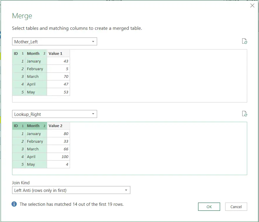
We start with the Left Anti Join Query. So, after Data/Get Data/Combine Queries/Merge, we get to the Merge window

After OK’ing that, we get this

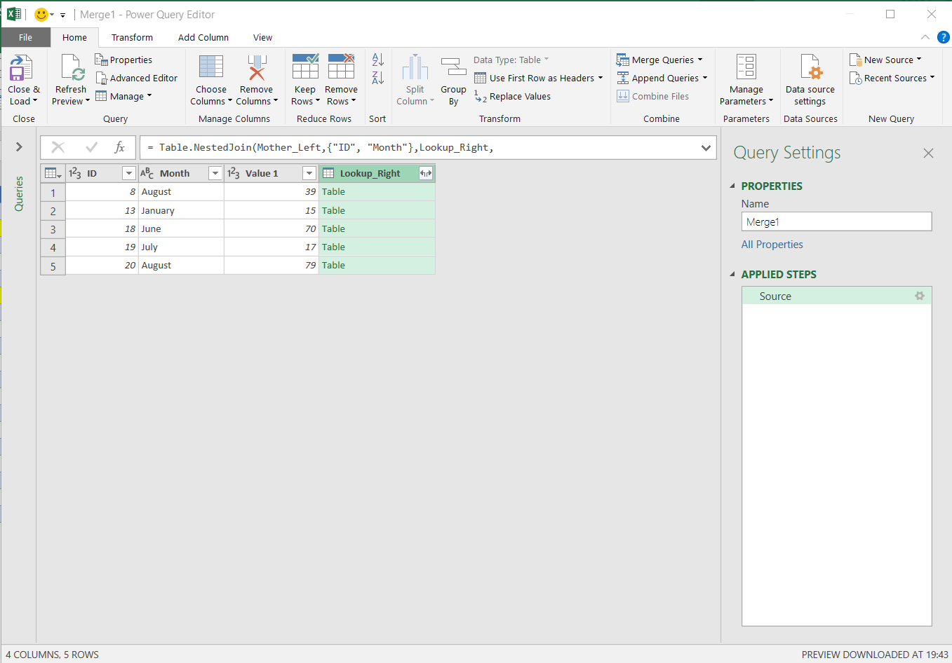
We then Rename the Query into LeftOutliers and get rid of the Lookup_Right column which contains nothing but null’s.

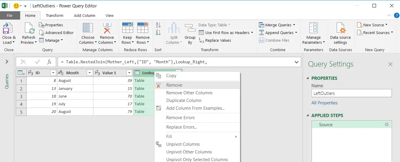
After we’re left with this, we select Home/Close & Load To… and choose Connection Only.

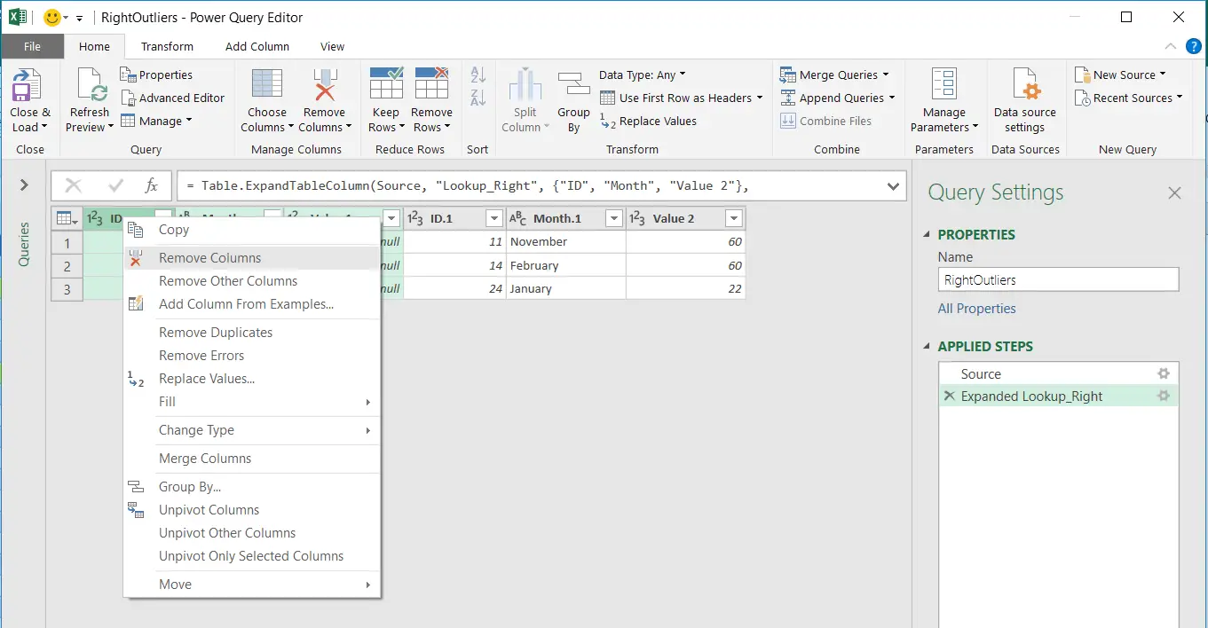
Then we repeat the process with the only difference being the Right Anti Join instead of a left one. We save this query as RightOutliers this time removing the first three columns since they are all nulls.

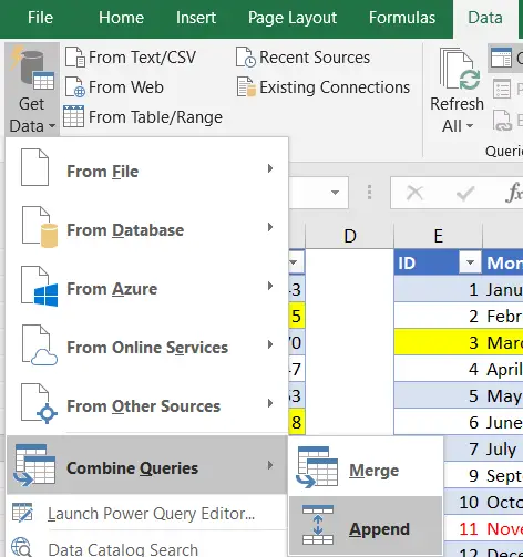
And now comes the final Query. We select Data/Get Data/Combine Queries/Append

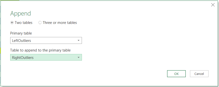
And choose to Combine LeftOutliers with RightOutliers

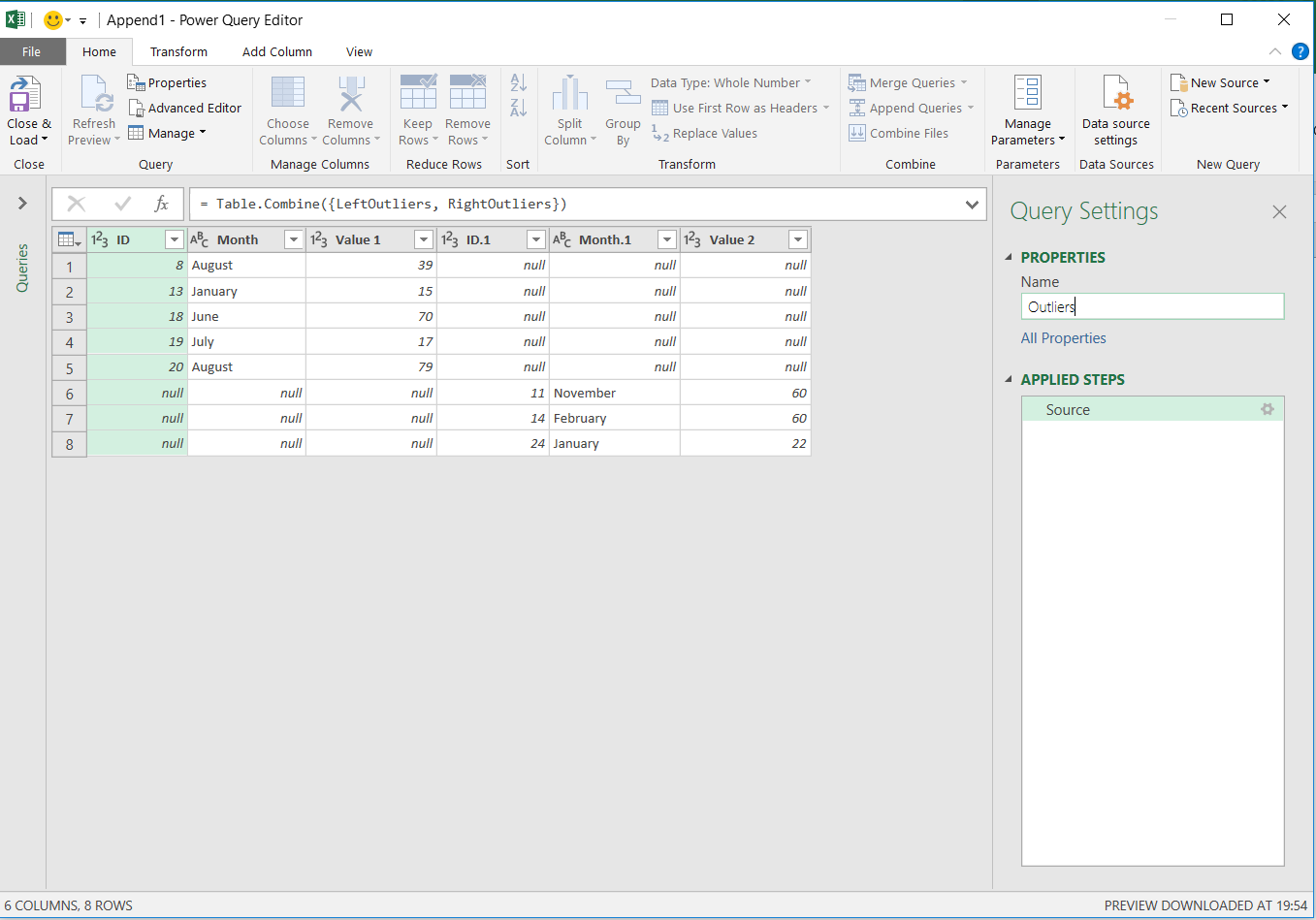
Hitting OK gives us exactly what we need, all Outliers from both tables.

2      Returning multiple Values

This one I’m extremely fond of. Excel has a tool called Remove Duplicates on the Data tab. It’s a brilliant tool and yet every time I show it at a training session, the desire for a tool that would only return duplicates immensely outweighs the potential enthusiasm over the Remove Duplicates tool. But now, with Power Query, you can easily get a list of your duplicates. This is how.

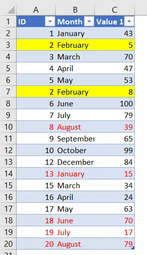
Let’s say we want to find all the duplicates from Mother_Left. That would be all the Yellow rows.

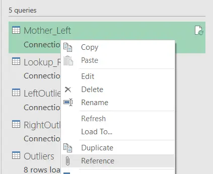
What we do is a reference of the Mother_Left query which we created in Part 1 (also part of the workbook you can download above)

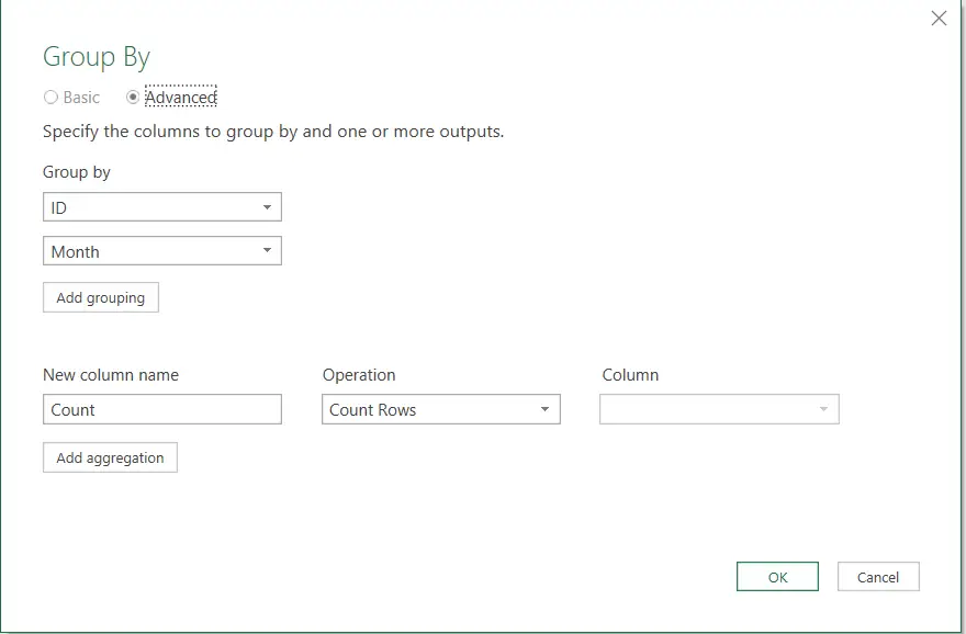
Now we select all the columns we wish to search duplicates by. In our case that’s ID and Month and select Home/Group By

We get this

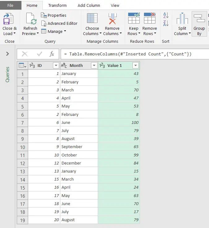
So we group by ID and Month and choose to Count Rows. Here’s the result

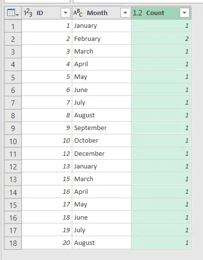
And after we filter that down to just those rows where Count is greater than one…

There it is… All our duplicates.

3      Give me the Vlookup Statistics

In November of 2017 I was speaking at the Bulgarian Excel Days Conference that was organized by Boriana Petrova (Excel MVP from Bulgaria). The title of my talk was The Vlookup Dashboard. And I was speaking about doing exactly what the last Title implies. It was a Power Query driven statistic of a “Vlookup” operation. I’m going to call it an operation because the dashboard itself didn’t include a single Vlookup. It was all Power Query Driven. And here are some of the things that you can do:

Number of Outliers in the Main Table and the lookup table. Number of duplicates. Number of successful “lookups” and practically anything you want. Let’s show a Dashboard of the number of Outliers.

So we’re going to use the LeftOutliers and the RightOutliers queries that we did in the first sample of this post and do a reference on them

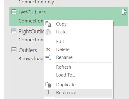
And then just do Transform/Statistics/Count Values

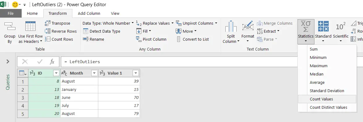
And we get a number as a result of our query and I will call this query LOutNum (as in Number of LeftOutliers)

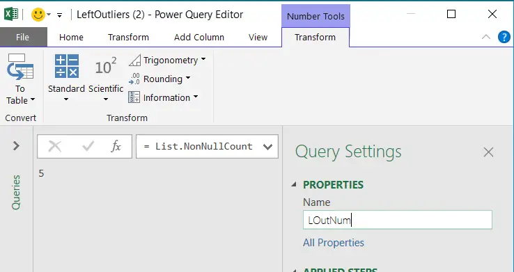
We just Close And Load To… and do a Connection only… Next we repeat the same thing for the RightOutliers query. Now we should have both…

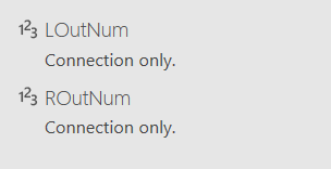
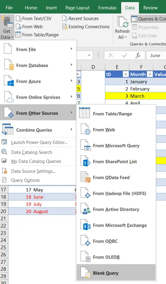
Now we create the reporting table… We go to Data/ Get Data / From Other Sources / Blank Query

Open the Advanced Editor

And write some crazy M code

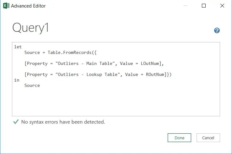
Source = Table.FromRecords({

[Property = "Outliers - Main Table", Value = LOutNum],

[Property = "Outliers - Lookup Table", Value = ROutNum]})

in

Source

It’s actually as simple as it gets. It’s manually creating a table with columns Property and Value, where we define properties manually and call values from the previous queries. And there it is…

The desired Vlookup Dashboard. Pure Brilliance!